Understanding LR Finder and Cyclic Learning Rates using Tensorflow 2

A group of us at work are following Jeremy Howard's Practical Deep Learning for Coders, v3. Basically we watch the videos on our own, and come together once a fortnight or so, to discuss things that seemed interesting and useful, or if someone has questions that others might then try to answer. One thing that's covered fairly early on in the course is how to use the Learning Rate Finder (LR Finder) tool that comes built-in with the fast.ai library (fastai/fastai on github). The fast.ai library builds on top of the Pytorch framework, and provides convenience functions that can make deep learning development simpler. A lot like what Keras did for Tensorflow, which incidentally is also the Deep Learning framework that I started with and confess being somewhat partial to, although nowadays I use the tf.keras (Tensorflow) port exclusively. So I figured that it would be interesting to see how to do this (LR Finding) with Keras.

The LR Finder is the brainchild of Leslie Smith, who has published two papers on it -- A disciplined approach to neural network hyperparameters: Part 1 -- Learning Rate, Batch Size, Momentum, and Weight Decay, and another jointly with Nicholay Topin, Super-Convergence: Very Fast Training of Neural Networks using Large Learning Rates. The LR Finder approach is able to predict, with only a few iterations of training, a range of learning rates that would be optimal for a given model/dataset combination. It does this by varying the learning rate across the training iterations, and observing the loss for each learning rate. The shape of the plot of loss against learning rates provides clues about the optimal range of learning rates, much like stock charts provides clues to future prices of the stock.

This in itself is a pretty big time savings, compared to running limited epochs of training with different learning rates to find the "best" one. But in addition to that, Smith also proposes using a Learning Rate Schedule he calls the Cyclic Learning Rate (CLR). In its simplest incarnation, the learning rate schedule for CLR looks a bit like an isoceles triangle. Assuming N epochs of training, and an optimum learning rate range predicted by the LR Finder plot (min_lr, max_lr), for the first N/2 epochs, the learning rate rises uniformly from min_lr to max_lr, and for about 90% of the next N/2 epochs, it falls uniformly from max_lr to min_lr, then for the last 10%, it falls uniformly from min_lr to 0. According to his experiments on a wide variety of standard model/dataset combinations, using the CLR schedule trains networks results in higher classification accuracy often with fewer epochs of training, compared to using static learning rates.

There is already a LR Finder and CLR schedule implementation for Keras, thanks to Somshubhra Majumdar (titu1994/keras-one-cycle), where both the LR Finder and CLR Schedule (called OneCycleLR here) are implemented as Keras callbacks. There is a decidedly Keras flavor to the implementation. For example, the LR Finder always runs for one epoch of training. However, there are advantages to using this implementation compared to rolling your own. For example, unlike the LearningRateScheduler callback built into Keras, the OneCycleLR callback also optionally allows the caller to schedule a Momentum Schedule along with a Learning Rate Schedule. Overall, it would take some effort to convert over to tf.keras, but probably not a whole lot.

At the other end of the spectrum is a Pytorch implementation from David Silva (davidtvs/pytorch-lr-finder), where the LR Finder is more of a standalone utility, which can predict the optimum range of learning rates given a model/dataset combination. I felt this approach was a bit cleaner in the sense that one can focus on what the LR finder does rather than try to think in terms of callback events.

So I decided to use the pytorch-lr-finder as a model to build a basic LR Finder of my own that works against tf.keras on Tensorflow 2, and try it out against a small standard network to see how it works. For the CLR scheduler, I decided to pass a homegrown version of the CLR schedule into the built in tf.keras LearningRateScheduler. This post will describe that experience. However, since this was mainly a learning exercise, the code has not been tested beyond what I describe here, so for your own work, you should probably stick to using the more robust implementations I referenced above.

The network I decided on was the LeNet network, proposed by Yann LeCun in 1995. The actual implementation is based on Wei Li's Keras implementation available on the BIGBALLON/cifar-10-cnn repository. The class is defined as follows, using the new imperative Chainer like syntax adopted by Pytorch and now Tensorflow 2. I had originally assumed, like many others, that this syntax was one of the features that Tensorflow 2 was adopting from Pytorch, but it turns out that they are both adopting it from Chainer, as this Twitter thread from François Chollet indicates. In any case, convergence is a good thing for framework users like me. Talking of tweets from François Chollet, if you are comfortable with Keras already, here is another Twitter thread which tells you pretty much everything you need to know to get started with Tensorflow 2.

1 2 3 4 5 6 7 8 9 10 11 12 13 14 15 16 17 18 19 20 21 22 23 24 25 26 27 28 29 30 31 32 33 34 35 36 37 38 39 40 41 42 43 44 45 46 47

class LeNetModel(tf.keras.Model): def __init__(self, **kwargs): super(LeNetModel, self).__init__(**kwargs) self.conv1 = tf.keras.layers.Conv2D( filters=6, kernel_size=(5, 5), padding="valid", activation="relu", kernel_initializer="he_normal", input_shape=(32, 32, 3)) self.pool1 = tf.keras.layers.MaxPooling2D( pool_size=(2, 2)) self.conv2 = tf.keras.layers.Conv2D( filters=16, kernel_size=(5, 5), padding="valid", activation="relu", kernel_initializer="he_normal") self.pool2 = tf.keras.layers.MaxPooling2D( pool_size=(2, 2), strides=(2, 2)) self.flat = tf.keras.layers.Flatten() self.dense1 = tf.keras.layers.Dense( units=120, activation="relu", kernel_initializer="he_normal") self.dense2 = tf.keras.layers.Dense( units=84, activation="relu", kernel_initializer="he_normal") self.dense3 = tf.keras.layers.Dense( units=10, activation="softmax", kernel_initializer="he_normal") def call(self, x): x = self.conv1(x) x = self.pool1(x) x = self.conv2(x) x = self.pool2(x) x = self.flat(x) x = self.dense1(x) x = self.dense2(x) x = self.dense3(x) return x

Here is the Keras summary view for those of you who prefer something more visual. If you were wondering how I got actual values in the Output Shape column with the code above, I didn't. As Tensorflow Issue# 25036 indicates, the call() method creates a non-static graph, and so model.summary() is unable to compute the output shapes. To generate the summary below, I rebuilt the model as a static graph using tf.keras.models.Sequential(). The code is fairly trivial so I don't include it here.

Model: "le_net_model"
_________________________________________________________________
Layer (type)                 Output Shape              Param #   
=================================================================
conv1 (Conv2D)               (None, 28, 28, 6)         456       
_________________________________________________________________
pool1 (MaxPooling2D)         (None, 14, 14, 6)         0         
_________________________________________________________________
conv2 (Conv2D)               (None, 10, 10, 16)        2416      
_________________________________________________________________
pool2 (MaxPooling2D)         (None, 5, 5, 16)          0         
_________________________________________________________________
flatten (Flatten)            (None, 400)               0         
_________________________________________________________________
dense1 (Dense)               (None, 120)               48120     
_________________________________________________________________
dense2 (Dense)               (None, 84)                10164     
_________________________________________________________________
dense3 (Dense)               (None, 10)                850       
=================================================================
Total params: 62,006
Trainable params: 62,006
Non-trainable params: 0
_________________________________________________________________

The dataset I used for the experiment was the CIFAR-10 dataset, a collection of 60K (32, 32, 3) color images (tiny images) in 10 different classes. The CIFAR-10 dataset is available via the tf.keras.datasets package. The function below downloads the data, preprocesses it appropriately for use by the network, and converts it into the tf.data.Dataset format that Tensorflow 2 likes. It will return datasets for training, validation, and test, with size 45K, 5K, and 10K images respectively.

1 2 3 4 5 6 7 8 9 10 11 12 13 14 15 16 17 18 19 20 21 22 23 24 25

def load_cifar10_data(batch_size): (xtrain, ytrain), (xtest, ytest) = tf.keras.datasets.cifar10.load_data() # scale data using MaxScaling xtrain = xtrain.astype(np.float32) / 255 xtest = xtest.astype(np.float32) / 255 # convert labels to categorical ytrain = tf.keras.utils.to_categorical(ytrain) ytest = tf.keras.utils.to_categorical(ytest) train_dataset = tf.data.Dataset.from_tensor_slices((xtrain, ytrain)) test_dataset = tf.data.Dataset.from_tensor_slices((xtest, ytest)) # take out 10% of train data as validation data, shuffle, and batch val_size = xtrain.shape[0] // 10 train_dataset = train_dataset.shuffle(10000) val_dataset = train_dataset.take(val_size).batch( batch_size, drop_remainder=True) train_dataset = train_dataset.skip(val_size).batch( batch_size, drop_remainder=True) test_dataset = test_dataset.shuffle(10000).batch( batch_size, drop_remainder=True) return train_dataset, val_dataset, test_dataset

I trained the model first using a learning rate of 0.001, which I picked up from the blog post CIFAR-10 Image Classification in Tensorflow by Park Chansung. The training code is just 5-6 lines of code that is very familiar to Keras developers - declare the model, compile the model with loss function and optimizer, then train it for a fixed number of epochs (10), and finally evaluate it against the held out test dataset.

1 2 3 4 5 6 7 8 9 10

model = LeNetModel() model.build(input_shape=(None, 32, 32, 3)) learning_rate = 0.001 optimizer = tf.keras.optimizers.SGD(learning_rate=learning_rate) loss_fn = tf.keras.losses.CategoricalCrossentropy() model.compile(loss=loss_fn, optimizer=optimizer, metrics=["accuracy"]) model.fit(train_dataset, epochs=10, validation_data=val_dataset) model.evaluate(test_dataset)

The output of this run is shown below. The first block is the output from the training run (model.fit()), and the last line is the output of the model.evaluate() call. As you can see, while the final accuracy values are not stellar, it is steadily increasing, so presumably we can expect good results given enough epochs of training. Also, the objective of this run was to create a baseline against which we will measure training runs with learning rates that we infer from our LR finder, described below.

Epoch 1/10
351/351 [==============================] - 12s 35ms/step - loss: 2.3043 - accuracy: 0.1105 - val_loss: 2.2936 - val_accuracy: 0.1170
Epoch 2/10
351/351 [==============================] - 12s 34ms/step - loss: 2.2816 - accuracy: 0.1276 - val_loss: 2.2801 - val_accuracy: 0.1330
Epoch 3/10
351/351 [==============================] - 12s 33ms/step - loss: 2.2682 - accuracy: 0.1464 - val_loss: 2.2668 - val_accuracy: 0.1442
Epoch 4/10
351/351 [==============================] - 11s 33ms/step - loss: 2.2517 - accuracy: 0.1620 - val_loss: 2.2474 - val_accuracy: 0.1621
Epoch 5/10
351/351 [==============================] - 12s 33ms/step - loss: 2.2254 - accuracy: 0.1856 - val_loss: 2.2141 - val_accuracy: 0.1893
Epoch 6/10
351/351 [==============================] - 12s 34ms/step - loss: 2.1810 - accuracy: 0.2117 - val_loss: 2.1601 - val_accuracy: 0.2226
Epoch 7/10
351/351 [==============================] - 12s 34ms/step - loss: 2.1144 - accuracy: 0.2421 - val_loss: 2.0856 - val_accuracy: 0.2526
Epoch 8/10
351/351 [==============================] - 12s 35ms/step - loss: 2.0363 - accuracy: 0.2641 - val_loss: 2.0116 - val_accuracy: 0.2714
Epoch 9/10
351/351 [==============================] - 12s 35ms/step - loss: 1.9704 - accuracy: 0.2841 - val_loss: 1.9583 - val_accuracy: 0.2901
Epoch 10/10
351/351 [==============================] - 13s 36ms/step - loss: 1.9243 - accuracy: 0.2991 - val_loss: 1.9219 - val_accuracy: 0.2985

78/78 [==============================] - 1s 13ms/step - loss: 1.9079 - accuracy: 0.3112

My version of the LR Finder presents an API similar to the pytorch-lr-finder, where you pass in the model, optimizer, loss function, and dataset to create an instance of LRFinder. You then make call range_test() on the LRFinder with the minimum and maximum boundaries for learning rate, and the number of iterations. This step is similar to the Learner.lr_find() call in fast.ai. The range_test() function will split the learning rate range into the specified number of iterations given by num_iter, and train the model with one batch with each learning rate, and record the loss. Finally, the plot() method will plot the losses against the learning rate. Since we are training at the batch level, we need to calculate losses and gradients ourselves, as seen in the train_step() function. The code for the LRFinder class is as follows. The main section (under if __name__ == "__main__") contains calling code using the LeNet model, CIFAR-10 dataset, the SGD optimizer, and the categorical cross-entropy loss function.

1 2 3 4 5 6 7 8 9 10 11 12 13 14 15 16 17 18 19 20 21 22 23 24 25 26 27 28 29 30 31 32 33 34 35 36 37 38 39 40 41 42 43 44 45 46 47 48 49 50 51 52 53 54 55 56 57 58 59 60 61 62 63 64 65 66 67 68 69 70 71 72 73 74 75 76 77 78 79 80 81 82 83 84 85 86 87 88 89 90 91 92 93 94 95

import matplotlib.pyplot as plt import numpy as np import tensorflow as tf class LRFinder(object): def __init__(self, model, optimizer, loss_fn, dataset): super(LRFinder, self).__init__() self.model = model self.optimizer = optimizer self.loss_fn = loss_fn self.dataset = dataset # placeholders self.lrs = None self.loss_values = None self.min_lr = None self.max_lr = None self.num_iters = None @tf.function def train_step(self, x, y, curr_lr): tf.keras.backend.set_value(self.optimizer.lr, curr_lr) with tf.GradientTape() as tape: # forward pass y_ = self.model(x) # external loss value for this batch loss = self.loss_fn(y, y_) # add any losses created during forward pass loss += sum(self.model.losses) # get gradients of weights wrt loss grads = tape.gradient(loss, self.model.trainable_weights) # update weights self.optimizer.apply_gradients(zip(grads, self.model.trainable_weights)) return loss def range_test(self, min_lr, max_lr, num_iters, debug): # create learning rate schedule self.min_lr = min_lr self.max_lr = max_lr self.num_iters = num_iters self.lrs = np.linspace( self.min_lr, self.max_lr, num=self.num_iters) # initialize loss_values self.loss_values = [] curr_lr = self.min_lr for step, (x, y) in enumerate(self.dataset): if step >= self.num_iters: break loss = self.train_step(x, y, curr_lr) self.loss_values.append(loss.numpy()) if debug: print("[DEBUG] Step {:d}, Loss {:.5f}, LR {:.5f}".format( step, loss.numpy(), self.optimizer.learning_rate.numpy())) curr_lr = self.lrs[step] def plot(self): plt.plot(self.lrs, self.loss_values) plt.xlabel("learning rate") plt.ylabel("loss") plt.title("Learning Rate vs Loss ({:.2e}, {:.2e}, {:d})" .format(self.min_lr, self.max_lr, self.num_iters)) plt.xscale("log") plt.grid() plt.show() if __name__ == "__main__": tf.random.set_seed(42) # model model = LeNetModel() model.build(input_shape=(None, 32, 32, 3)) # optimizer optimizer = tf.keras.optimizers.SGD() # loss_fn loss_fn = tf.keras.losses.CategoricalCrossentropy() # dataset batch_size = 128 dataset, _, _ = load_cifar10_data(batch_size) # min_lr, max_lr # min_lr = 1e-6 # max_lr = 3 min_lr = 1e-2 max_lr = 1 # compute num_iters (Keras fit-one-cycle used 1 epoch by default) dataset_len = 45000 batch_size = 128 num_iters = dataset_len // batch_size # declare LR Finder lr_finder = LRFinder(model, optimizer, loss_fn, dataset) lr_finder.range_test(min_lr, max_lr, num_iters, debug=True) lr_finder.plot()

We first ran the LRFinder for a relatively large learning rate range from 1e-6 to 3. This gives us the chart on the left below. For the CLR schedule, the minimum LR for our range is where the loss starts descending, and the maximum LR is where the loss stops descending or becomes ragged. My charts are not as clean as those shown in the two projects referenced, but we can still infer that these boundaries are 1e-6 and about 3e-1. The chart on the right below is the plot of LR vs Loss on a smaller range (1e-2 and 1) to help see the chart in greater detail. We also see that the LR with minimum loss is about 3e-1.


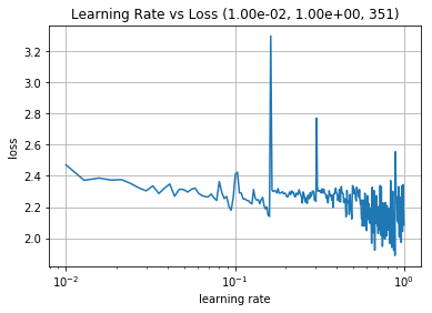Based on this, my first experiment is to try and train the network with the larger best learning rate (3e-1) we found from the LR Finder, and see if it trains better over 10 epochs than my previous attempt. The only thing we have changed here from the previous training code block above is to replace learning_rate from 0.001 to 0.3. Here are the results of 10 epochs of training, followed by evaluation on the held out test set.

Epoch 1/10
351/351 [==============================] - 12s 36ms/step - loss: 2.1572 - accuracy: 0.1664 - val_loss: 1.9966 - val_accuracy: 0.2590
Epoch 2/10
351/351 [==============================] - 12s 34ms/step - loss: 1.8960 - accuracy: 0.2979 - val_loss: 1.7568 - val_accuracy: 0.3732
Epoch 3/10
351/351 [==============================] - 12s 35ms/step - loss: 1.7456 - accuracy: 0.3642 - val_loss: 1.6556 - val_accuracy: 0.3984
Epoch 4/10
351/351 [==============================] - 12s 35ms/step - loss: 1.6634 - accuracy: 0.4021 - val_loss: 1.6050 - val_accuracy: 0.4331
Epoch 5/10
351/351 [==============================] - 12s 35ms/step - loss: 1.5993 - accuracy: 0.4213 - val_loss: 1.6906 - val_accuracy: 0.3858
Epoch 6/10
351/351 [==============================] - 12s 36ms/step - loss: 1.5244 - accuracy: 0.4484 - val_loss: 1.5754 - val_accuracy: 0.4399
Epoch 7/10
351/351 [==============================] - 13s 36ms/step - loss: 1.4568 - accuracy: 0.4749 - val_loss: 1.4996 - val_accuracy: 0.4712
Epoch 8/10
351/351 [==============================] - 13s 36ms/step - loss: 1.3894 - accuracy: 0.4971 - val_loss: 1.4854 - val_accuracy: 0.4786
Epoch 9/10
351/351 [==============================] - 12s 35ms/step - loss: 1.3323 - accuracy: 0.5207 - val_loss: 1.4527 - val_accuracy: 0.4950
Epoch 10/10
351/351 [==============================] - 12s 36ms/step - loss: 1.2817 - accuracy: 0.5411 - val_loss: 1.4320 - val_accuracy: 0.5068

78/78 [==============================] - 1s 12ms/step - loss: 1.4477 - accuracy: 0.4920

Clearly, the larger learning rate is helping the network achieve better performance, although it does seem (at least around epoch 3) that it may be slightly too large. Accuracy numbers on the held out test set jumped from 0.3112 to 0.4920. So overall it seems to be helping. So even if we just use the LR Finder to find the "best" learning rate, this is still cheaper than doing multiple training runs of a few epochs each.

Finally, we will try using a Cyclic Learning Rate (CLR) schedule using the learning rate boundaries (1e-6, 3e-1). The code for this is shown below. The clr_schedule() function produces a triangular learning rate schedule which rises for the first 5 epochs (in our case) from the minimum specified learning rate to the maximum, then falls from the maximum to the minimum for the next 4 epochs, and finally falls to half the minimum for the last epoch. This is analogous to the Learner.fit_one_cycle() call in fast.ai. The clr_schedule function is passed to the LearningRateScheduler callback, which is then called by the model training loop via the callback parameter in the fit() function call. Here is the code.

1 2 3 4 5 6 7 8 9 10 11 12 13 14 15 16 17 18 19 20 21 22 23 24 25 26 27 28 29 30 31 32 33 34 35 36 37 38

import matplotlib.pyplot as plt import numpy as np import tensorflow as tf def clr_schedule(epoch): num_epochs = 10 mid_pt = int(num_epochs * 0.5) last_pt = int(num_epochs * 0.9) min_lr, max_lr = 1e-6, 3e-1 if epoch <= mid_pt: return min_lr + epoch * (max_lr - min_lr) / mid_pt elif epoch > mid_pt and epoch <= last_pt: return max_lr - ((epoch - mid_pt) * (max_lr - min_lr)) / mid_pt else: return min_lr / 2 # plot the points # epochs = [x+1 for x in np.arange(10)] # clrs = [clr_schedule(x) for x in epochs] # plt.plot(epochs, clrs) # plt.show() batch_size = 128 train_dataset, val_dataset, test_dataset = load_cifar10_data(batch_size) model = LeNetModel() min_lr = 1e-6 max_lr = 3e-1 optimizer = tf.keras.optimizers.SGD(learning_rate=min_lr) loss_fn = tf.keras.losses.CategoricalCrossentropy() lr_scheduler = tf.keras.callbacks.LearningRateScheduler(clr_schedule) model.compile(loss=loss_fn, optimizer=optimizer, metrics=["accuracy"]) model.fit(train_dataset, epochs=10, validation_data=val_dataset, callbacks=[lr_scheduler]) model.evaluate(test_dataset)

And here are the results of training the LeNet model with the CIFAR-10 dataset for 10 epochs, and evaluating on the held out test set. As you can see, the evaluation accuracy on the held out test set has jumped further from 0.4920 to 0.5469.

Epoch 1/10
351/351 [==============================] - 13s 36ms/step - loss: 2.7753 - accuracy: 0.0993 - val_loss: 2.7627 - val_accuracy: 0.1060
Epoch 2/10
351/351 [==============================] - 12s 34ms/step - loss: 2.0131 - accuracy: 0.2097 - val_loss: 2.0829 - val_accuracy: 0.2634
Epoch 3/10
351/351 [==============================] - 12s 34ms/step - loss: 1.8321 - accuracy: 0.3106 - val_loss: 1.7187 - val_accuracy: 0.3718
Epoch 4/10
351/351 [==============================] - 12s 35ms/step - loss: 1.7100 - accuracy: 0.3648 - val_loss: 1.7484 - val_accuracy: 0.3928
Epoch 5/10
351/351 [==============================] - 12s 36ms/step - loss: 1.5779 - accuracy: 0.4209 - val_loss: 1.6188 - val_accuracy: 0.4087
Epoch 6/10
351/351 [==============================] - 13s 36ms/step - loss: 1.5451 - accuracy: 0.4300 - val_loss: 1.5704 - val_accuracy: 0.4377
Epoch 7/10
351/351 [==============================] - 12s 35ms/step - loss: 1.3597 - accuracy: 0.5063 - val_loss: 1.3742 - val_accuracy: 0.5014
Epoch 8/10
351/351 [==============================] - 12s 36ms/step - loss: 1.2383 - accuracy: 0.5484 - val_loss: 1.3620 - val_accuracy: 0.5204
Epoch 9/10
351/351 [==============================] - 12s 35ms/step - loss: 1.1379 - accuracy: 0.5856 - val_loss: 1.3336 - val_accuracy: 0.5391
Epoch 10/10
351/351 [==============================] - 12s 35ms/step - loss: 1.0564 - accuracy: 0.6130 - val_loss: 1.3008 - val_accuracy: 0.5557

78/78 [==============================] - 1s 13ms/step - loss: 1.3043 - accuracy: 0.5469

This indicates that the LR Finder and CLR schedule seem like good ideas to try when training your models, especially when using non-adaptive optimizers such as SGD.

I tried the same sequence of experiments with the Adam optimizer, and I got better results (test accuracy: 0.5908) using a fixed learning rate of 1e-3 for the first training run. Thereafter, based on the LR Finder reporting a learning rate range of (1e-6, 1e-1), the next two experiments using the best learning rate and CLR schedule both produced accuracies of about 0.1 (i.e., close to random for 10-class classifier). I wasn't too surprised, since I figured that the CLR schedule probably interfered with Adam's own learning rate schedule. However, according to this tweet from Jeremy Howard, the LR Finder can be used with the Adam optimizer as well. Given that he has probably conducted many more experiments around this than I have, and the fast.ai Learner.lr_find() code is more robust and heavily tested than my homegrown implementation, he is very likely right, and my results are an anomaly.

That's all I have for today. Thanks for staying with me so far. I learned a lot from implementing this code, and hopefully you learned a few things from reading this as well. Hopefully, this gives you some ideas for building an LR Finder for Tensorflow 2 that can be used easily by end-users -- if you do end up building one, please let me know, will be happy to link to your site/repository and recommend it to other readers.