First steps with Pytorch Lightning

Some time back, Quora routed a "Keras vs. Pytorch" question to me, which I decided to ignore because it seemed too much like flamebait to me. Couple of weeks back, after discussions with colleagues and (professional) acquaintances who had tried out libraries like Catalyst, Ignite, and Lightning, I decided to get on the Pytorch boilerplate elimination train as well, and tried out Pytorch Lightning. As I did so, my thoughts inevitably went back to the Quora question, and I came to the conclusion that, in their current form, the two libraries and their respective ecosystems are more similar than they are different, and that there is no technological reason to choose one over the other. Allow me to explain.

Neural networks learn using Gradient Descent. The central idea behind Gradient Descent can be neatly encapsulated in the equation below (extracted from the same linked Gradient Descent article), and is referred to as the "training loop". Of course, there are other aspects of neural networks, such as model and data definition, but it is the training loop where the differences in the earlier versions of the two libraries and their subsequent coming together are most apparent. So I will mostly talk about the training loop here.

Keras was initially conceived of as a high level API over the low level graph based APIs from Theano and Tensorflow. Graph APIs allow the user to first define the computation graph and then execute it. Once the graph is defined, the library will attempt to build the most efficient representation for the graph before execution. This makes the execution more efficient, but adds a lot of boilerplate to the code, and makes it harder to debug if something goes wrong. The biggest success of Keras in my opinion is its ability to hide the graph API almost completely behind an elegant API. In particular, its "training loop" looks like this:

1 2	model.compile(optimizer=optimizer, loss=loss_fn, metrics=[train_acc]) model.fit(Xtrain, ytrain, epochs=epochs, batch_size=batch_size)

Of course, the fit method has many other parameters as well, but at its most complex, it is a single line call. And, this is probably all that is needed for most simple cases. However, as networks get slightly more complex, with maybe multiple models or loss functions, or custom update rules, the only option for Keras used to be to drop down to the underlying Tensorflow or Theano code. In these situations, Pytorch appears really attractive, with the power, simplicity, and readability of its training loop.

1 2 3 4 5 6 7 8 9 10 11 12 13 14 15

dataloader = DataLoader(Xtrain, batch_size=batch_size) for epoch in epochs: for batch in dataloader: X, y = batch logits = model(X) loss = loss_fn(logits, y) loss.backward() optimizer.step() optimizer.zero_grad() # aggregate metrics train_acc(logits, loss) # evaluate validation loss, etc.

However, with the release of Tensorflow 2.x, which included Keras as its default API through the tf.keras package, it is now possible to do something identical with Keras and Tensorflow as well.

1 2 3 4 5 6 7 8 9 10 11 12

dataset = Dataset.from_tensor_slices(Xtrain).batch(batch_size) for epoch in epochs: for batch in dataset: X, y = batch with tf.GradientTape as tape: logits = model(X) loss = loss_fn(y_pred=logits, y_true=y) grads = tape.gradient(loss, model.trainable_weights) optimizer.apply_gradients(zip(grads, model.trainable_weights)) # aggregate metrics train_acc(logits, y)

In both cases, developers accept having to deal with some amount of boilerplate in return for additional power and flexibility. The approach taken by each of the three Pytorch add-on libraries I listed earlier, including Pytorch Lightning, is to create a Trainer object. The trainer models the training loop as an event loop with hooks into which specific functionality can be injected as callbacks. Functionality in these callbacks would be executed at specific points in the training loop. So a partial LightningModule subclass for our use case would look something like this, see the Pytorch Lightning Documentation or my code examples below for more details.

1 2 3 4 5 6 7 8 9 10 11 12 13 14 15 16 17 18 19 20

class MyLightningModel(pl.LightningModule): def __init__(self, args): # same as Pytorch nn.Module subclass __init__() def forward(self, x): # same as Pytorch nn.Module subclass forward() def training_step(self, batch, batch_idx): x, y = batch logits = self.forward(x) loss = loss_fn(logits, y) acc = self.train_acc(logits, y) return loss def configure_optimizers(self): return self.optimizer model = MyLightningModel() trainer = pl.Trainer(gpus=1) trainer.fit(model, dataloader)

If you think about it, this event loop strategy used by Lightning's trainer.fit() is pretty much how Keras manages to convert its training loop to a single line model.fit() call as well, its many parameters acting as the callbacks that control the training behavior. Pytorch Lightning is just a bit more explicit (and okay, a bit more verbose) about it. In effect, both libraries have solutions that address the other's pain points, so the only reason you would choose one or the other is personal or corporate preference.

In addition to callbacks for each of training, validation, and test steps, there are additional callbacks for each of these steps that will be called at the end of each step and epoch, for example: training_epoch_end() and training_step_end(). Another nice side effect of adopting something like Pytorch Lightning is that you get some of the default functionality of the event loop for free. For example, logging is done to Tensorboard by default, and progress bars are controlled using TQDM. Finally, (and that is the raison d'etre for Pytorch Lightning from the point of view of its developers) it helps you organize your Pytorch code.

To get familiar with Pytorch Lightning, I took three of my old notebooks, each dealing with training one major type of Neural Network architecture (from the old days) -- a fully connected, convolutional, and recurrent network, and converted it to use Pytorch Lightning. You may find it useful to look at, in addition to Pytorch Lightning's extensive documentation, including links to them below.

• Fully Connected Network (FCN) Example (with Pytorch and Pytorch + Lightning)
• Convolutional Network (CNN) Example (with Pytorch and Pytorch + Lightning).
• Recurrent Network (RNN) Example (with Pytorch and Pytorch + Lightning).

ODSC trip report and Keras Tutorial

I attended ODSC (Open Data Science Conference) West 2020 end of last month. I also presented Keras from Soup to Nuts -- an example driven tutorial there, a 3-hour tutorial on Keras. Like other conferences this year, the event was all-virtual. Having attended one other all-virtual conference this year (Knowledge Discovery and Data Mining (KDD) 2020 and being part of organizing another (an in-house conference), I can appreciate how much work it took to pull it off. As with the other conferences, I continue to be impressed at how effortless it all appears to be from the point of view of both speaker and attendee, so kudos to the ODSC organizers and volunteers for a job well done!

In this post, I want to cover my general impressions about the conference for readers of this blog. Content seems similar to PyData, except that not all talks here are based on Python (or Julia or R) related. As with PyData, the content is mostly targeted at data scientists in industry, with a few talks that are more academic, based on the presenter's own research. I think there is also more coverage on the career related aspects of Data Science than PyData. I also thought that there was more content here than in typical PyData conferences -- the conference was 4 days long (Monday to Friday) and multi-track, with workshops and presentations. The variety of content feels a bit like KDD but with less academic rigor. Overall, the content is high-quality, and if you enjoy attending PyData conferences, you will find more than enough talks and workshops here to hold your interest through the duration of the conference.

Pricing is also a bit steep compared to KDD and PyData, although there seem to be deep discounts available if you qualify. You have to contact the organizers for details about the discounts. Fortunately I didn't have to worry about that since I was presenting and my ticket was complimentary.

Like KDD and unlike PyData, OSDC also does not share talk recordings with the public after the conference. Speakers sometimes do share their slides and github repositories, so hopefully you will find these resources for the talks I list below. Because my internal conference (the one I was part of the organizing team for) was scheduled the very next week, I could not spend as much time at ODSC as I would have liked, so there were many talks that I would have liked to attend but I didn't. Here is the full schedule (until the link is repurposed for the 2021 conference).

• Evaluating and Testing Natural Language Processing Models -- interesting talk about generating adversarial examples to test Natural Language Processing (NLP) models, to gain insight into the inner workings of the model. The presenter is co-author of a paper titled Generating Natural Adversarial Examples.
• Natural Language Processing with Pytorch -- NLP tutorial aimed mostly at beginners, covers a lot of traditional techniques to establish good baselines, followed by some Pytorch examples on Sentiment Analysis and Summarization. This was a 3 hour tutorial (like the one I did), and had labs. Here is the github repository for the labs.
• Learning with Limited Labels -- I was interested in this from a NLP point of view, but the techniques covered were almost exclusively for Computer Vision (CV) problems. I enjoyed the talk though, I thought the examples covered were useful techniques for CV problems.
• Transfer Learning in NLP -- fairly high level survey of transfer learning in NLP, before and after BERT (and other transformers). If you haven't been following the field closely, this is a good refresher.
• Accelerating NLP Model Training and Deployment with Pytorch -- covers, among other things, how to write out and deploy trained transformer based models using the ONNX format. I thought this was quite interesting.
• Building Content Embeddings with Self Supervised Learning -- the presenters describe building vectors representing tweets based on random walks through the Twitter follower graph. These vectors can be used for recommending content from one Twitter user to another.
• A Comparison of Topic Modeling Methods in Python -- good notebook based talk on applying different topic modeling techniques (K-Means, LDA, and NMF) to the same dataset, and using different evaluation metrics to evaluate their quality.
• Machine Learning in Biology and Medicine -- good presentation with examples of applying ML techniques to genomics and Electronic Medical Records.

As I mentioned earlier already, I also presented a 3 hour tutorial on Keras, so I wanted to cover that in slightly greater detail for readers here as well. As implied by the name, and the talk abstract, the tutorial tries to teach participants enough Keras to become advanced Keras programmers, and assumes only some Python programming experience as a pre-requisite. Clearly 3 hours is not enough time, so the notebooks are deliberately short on theory and heavy on examples. I organized the tutorial into 3 45-minute sessions, with exercises at the end of the first two, but we ended up just running through the exercise solutions instead because of time constraints.

The tutorial materials are just a collection of Colab notebooks that are available at my sujitpal/keras-tutorial-odsc2020 github repository. The project README provides additional information about what each notebook contains. Each notebook is numbered with the session and sequence within each session. There are two notebooks called exercise 1 and 2, and corresponding solution notebooks titled exercise_1_solved and exercise_2_solved.

Keras started life as an easy to use high level API to Theano and Tensorflow, but has since been subsumed into Tensorflow 2.x as its default API. I was among those who learned Keras in its first incarnation, when certain things were just impossible to do in Keras, and the only option was to drop down to Tensorflow 1.x's two-step model (create compute graph and then run it with data). In many cases, Pytorch provided simpler ways to do the same thing, so for complex models I found myself increasingly gravitating towards Pytorch. I did briefly look at Keras (now tf.keras) and Tensorflow 2.0-alpha while co-authoring the Deep Learning with Tensorflow 2 and Keras book, but the software was new and there was not a whole lot information available at the time.

My point of mentioning all this is to acknowledge that I ended up learning a bit of advanced Keras myself as well when building the last few notebooks. Depending on where you are with Keras, you might find them interesting as well. Some of the interesting examples covered (according to me) are Sequence to Sequence models with and without attention, using transformers from the Huggingface Transformers library in your Keras models, using Cyclic Learning Rates and LR Finder, and distributed training across multiple GPUs and TPU. I am actually quite pleasantly surprised at how much more you can do with tf.keras with respect to the underlying Tensorflow framework, and I think you will be too (if you aren't already).

Understanding LR Finder and Cyclic Learning Rates using Tensorflow 2

A group of us at work are following Jeremy Howard's Practical Deep Learning for Coders, v3. Basically we watch the videos on our own, and come together once a fortnight or so, to discuss things that seemed interesting and useful, or if someone has questions that others might then try to answer. One thing that's covered fairly early on in the course is how to use the Learning Rate Finder (LR Finder) tool that comes built-in with the fast.ai library (fastai/fastai on github). The fast.ai library builds on top of the Pytorch framework, and provides convenience functions that can make deep learning development simpler. A lot like what Keras did for Tensorflow, which incidentally is also the Deep Learning framework that I started with and confess being somewhat partial to, although nowadays I use the tf.keras (Tensorflow) port exclusively. So I figured that it would be interesting to see how to do this (LR Finding) with Keras.

The LR Finder is the brainchild of Leslie Smith, who has published two papers on it -- A disciplined approach to neural network hyperparameters: Part 1 -- Learning Rate, Batch Size, Momentum, and Weight Decay, and another jointly with Nicholay Topin, Super-Convergence: Very Fast Training of Neural Networks using Large Learning Rates. The LR Finder approach is able to predict, with only a few iterations of training, a range of learning rates that would be optimal for a given model/dataset combination. It does this by varying the learning rate across the training iterations, and observing the loss for each learning rate. The shape of the plot of loss against learning rates provides clues about the optimal range of learning rates, much like stock charts provides clues to future prices of the stock.

This in itself is a pretty big time savings, compared to running limited epochs of training with different learning rates to find the "best" one. But in addition to that, Smith also proposes using a Learning Rate Schedule he calls the Cyclic Learning Rate (CLR). In its simplest incarnation, the learning rate schedule for CLR looks a bit like an isoceles triangle. Assuming N epochs of training, and an optimum learning rate range predicted by the LR Finder plot (min_lr, max_lr), for the first N/2 epochs, the learning rate rises uniformly from min_lr to max_lr, and for about 90% of the next N/2 epochs, it falls uniformly from max_lr to min_lr, then for the last 10%, it falls uniformly from min_lr to 0. According to his experiments on a wide variety of standard model/dataset combinations, using the CLR schedule trains networks results in higher classification accuracy often with fewer epochs of training, compared to using static learning rates.

There is already a LR Finder and CLR schedule implementation for Keras, thanks to Somshubhra Majumdar (titu1994/keras-one-cycle), where both the LR Finder and CLR Schedule (called OneCycleLR here) are implemented as Keras callbacks. There is a decidedly Keras flavor to the implementation. For example, the LR Finder always runs for one epoch of training. However, there are advantages to using this implementation compared to rolling your own. For example, unlike the LearningRateScheduler callback built into Keras, the OneCycleLR callback also optionally allows the caller to schedule a Momentum Schedule along with a Learning Rate Schedule. Overall, it would take some effort to convert over to tf.keras, but probably not a whole lot.

At the other end of the spectrum is a Pytorch implementation from David Silva (davidtvs/pytorch-lr-finder), where the LR Finder is more of a standalone utility, which can predict the optimum range of learning rates given a model/dataset combination. I felt this approach was a bit cleaner in the sense that one can focus on what the LR finder does rather than try to think in terms of callback events.

So I decided to use the pytorch-lr-finder as a model to build a basic LR Finder of my own that works against tf.keras on Tensorflow 2, and try it out against a small standard network to see how it works. For the CLR scheduler, I decided to pass a homegrown version of the CLR schedule into the built in tf.keras LearningRateScheduler. This post will describe that experience. However, since this was mainly a learning exercise, the code has not been tested beyond what I describe here, so for your own work, you should probably stick to using the more robust implementations I referenced above.

The network I decided on was the LeNet network, proposed by Yann LeCun in 1995. The actual implementation is based on Wei Li's Keras implementation available on the BIGBALLON/cifar-10-cnn repository. The class is defined as follows, using the new imperative Chainer like syntax adopted by Pytorch and now Tensorflow 2. I had originally assumed, like many others, that this syntax was one of the features that Tensorflow 2 was adopting from Pytorch, but it turns out that they are both adopting it from Chainer, as this Twitter thread from François Chollet indicates. In any case, convergence is a good thing for framework users like me. Talking of tweets from François Chollet, if you are comfortable with Keras already, here is another Twitter thread which tells you pretty much everything you need to know to get started with Tensorflow 2.

1 2 3 4 5 6 7 8 9 10 11 12 13 14 15 16 17 18 19 20 21 22 23 24 25 26 27 28 29 30 31 32 33 34 35 36 37 38 39 40 41 42 43 44 45 46 47

class LeNetModel(tf.keras.Model): def __init__(self, **kwargs): super(LeNetModel, self).__init__(**kwargs) self.conv1 = tf.keras.layers.Conv2D( filters=6, kernel_size=(5, 5), padding="valid", activation="relu", kernel_initializer="he_normal", input_shape=(32, 32, 3)) self.pool1 = tf.keras.layers.MaxPooling2D( pool_size=(2, 2)) self.conv2 = tf.keras.layers.Conv2D( filters=16, kernel_size=(5, 5), padding="valid", activation="relu", kernel_initializer="he_normal") self.pool2 = tf.keras.layers.MaxPooling2D( pool_size=(2, 2), strides=(2, 2)) self.flat = tf.keras.layers.Flatten() self.dense1 = tf.keras.layers.Dense( units=120, activation="relu", kernel_initializer="he_normal") self.dense2 = tf.keras.layers.Dense( units=84, activation="relu", kernel_initializer="he_normal") self.dense3 = tf.keras.layers.Dense( units=10, activation="softmax", kernel_initializer="he_normal") def call(self, x): x = self.conv1(x) x = self.pool1(x) x = self.conv2(x) x = self.pool2(x) x = self.flat(x) x = self.dense1(x) x = self.dense2(x) x = self.dense3(x) return x

Here is the Keras summary view for those of you who prefer something more visual. If you were wondering how I got actual values in the Output Shape column with the code above, I didn't. As Tensorflow Issue# 25036 indicates, the call() method creates a non-static graph, and so model.summary() is unable to compute the output shapes. To generate the summary below, I rebuilt the model as a static graph using tf.keras.models.Sequential(). The code is fairly trivial so I don't include it here.

Model: "le_net_model"
_________________________________________________________________
Layer (type)                 Output Shape              Param #   
=================================================================
conv1 (Conv2D)               (None, 28, 28, 6)         456       
_________________________________________________________________
pool1 (MaxPooling2D)         (None, 14, 14, 6)         0         
_________________________________________________________________
conv2 (Conv2D)               (None, 10, 10, 16)        2416      
_________________________________________________________________
pool2 (MaxPooling2D)         (None, 5, 5, 16)          0         
_________________________________________________________________
flatten (Flatten)            (None, 400)               0         
_________________________________________________________________
dense1 (Dense)               (None, 120)               48120     
_________________________________________________________________
dense2 (Dense)               (None, 84)                10164     
_________________________________________________________________
dense3 (Dense)               (None, 10)                850       
=================================================================
Total params: 62,006
Trainable params: 62,006
Non-trainable params: 0
_________________________________________________________________

The dataset I used for the experiment was the CIFAR-10 dataset, a collection of 60K (32, 32, 3) color images (tiny images) in 10 different classes. The CIFAR-10 dataset is available via the tf.keras.datasets package. The function below downloads the data, preprocesses it appropriately for use by the network, and converts it into the tf.data.Dataset format that Tensorflow 2 likes. It will return datasets for training, validation, and test, with size 45K, 5K, and 10K images respectively.

1 2 3 4 5 6 7 8 9 10 11 12 13 14 15 16 17 18 19 20 21 22 23 24 25

def load_cifar10_data(batch_size): (xtrain, ytrain), (xtest, ytest) = tf.keras.datasets.cifar10.load_data() # scale data using MaxScaling xtrain = xtrain.astype(np.float32) / 255 xtest = xtest.astype(np.float32) / 255 # convert labels to categorical ytrain = tf.keras.utils.to_categorical(ytrain) ytest = tf.keras.utils.to_categorical(ytest) train_dataset = tf.data.Dataset.from_tensor_slices((xtrain, ytrain)) test_dataset = tf.data.Dataset.from_tensor_slices((xtest, ytest)) # take out 10% of train data as validation data, shuffle, and batch val_size = xtrain.shape[0] // 10 train_dataset = train_dataset.shuffle(10000) val_dataset = train_dataset.take(val_size).batch( batch_size, drop_remainder=True) train_dataset = train_dataset.skip(val_size).batch( batch_size, drop_remainder=True) test_dataset = test_dataset.shuffle(10000).batch( batch_size, drop_remainder=True) return train_dataset, val_dataset, test_dataset

I trained the model first using a learning rate of 0.001, which I picked up from the blog post CIFAR-10 Image Classification in Tensorflow by Park Chansung. The training code is just 5-6 lines of code that is very familiar to Keras developers - declare the model, compile the model with loss function and optimizer, then train it for a fixed number of epochs (10), and finally evaluate it against the held out test dataset.

1 2 3 4 5 6 7 8 9 10

model = LeNetModel() model.build(input_shape=(None, 32, 32, 3)) learning_rate = 0.001 optimizer = tf.keras.optimizers.SGD(learning_rate=learning_rate) loss_fn = tf.keras.losses.CategoricalCrossentropy() model.compile(loss=loss_fn, optimizer=optimizer, metrics=["accuracy"]) model.fit(train_dataset, epochs=10, validation_data=val_dataset) model.evaluate(test_dataset)

The output of this run is shown below. The first block is the output from the training run (model.fit()), and the last line is the output of the model.evaluate() call. As you can see, while the final accuracy values are not stellar, it is steadily increasing, so presumably we can expect good results given enough epochs of training. Also, the objective of this run was to create a baseline against which we will measure training runs with learning rates that we infer from our LR finder, described below.

Epoch 1/10
351/351 [==============================] - 12s 35ms/step - loss: 2.3043 - accuracy: 0.1105 - val_loss: 2.2936 - val_accuracy: 0.1170
Epoch 2/10
351/351 [==============================] - 12s 34ms/step - loss: 2.2816 - accuracy: 0.1276 - val_loss: 2.2801 - val_accuracy: 0.1330
Epoch 3/10
351/351 [==============================] - 12s 33ms/step - loss: 2.2682 - accuracy: 0.1464 - val_loss: 2.2668 - val_accuracy: 0.1442
Epoch 4/10
351/351 [==============================] - 11s 33ms/step - loss: 2.2517 - accuracy: 0.1620 - val_loss: 2.2474 - val_accuracy: 0.1621
Epoch 5/10
351/351 [==============================] - 12s 33ms/step - loss: 2.2254 - accuracy: 0.1856 - val_loss: 2.2141 - val_accuracy: 0.1893
Epoch 6/10
351/351 [==============================] - 12s 34ms/step - loss: 2.1810 - accuracy: 0.2117 - val_loss: 2.1601 - val_accuracy: 0.2226
Epoch 7/10
351/351 [==============================] - 12s 34ms/step - loss: 2.1144 - accuracy: 0.2421 - val_loss: 2.0856 - val_accuracy: 0.2526
Epoch 8/10
351/351 [==============================] - 12s 35ms/step - loss: 2.0363 - accuracy: 0.2641 - val_loss: 2.0116 - val_accuracy: 0.2714
Epoch 9/10
351/351 [==============================] - 12s 35ms/step - loss: 1.9704 - accuracy: 0.2841 - val_loss: 1.9583 - val_accuracy: 0.2901
Epoch 10/10
351/351 [==============================] - 13s 36ms/step - loss: 1.9243 - accuracy: 0.2991 - val_loss: 1.9219 - val_accuracy: 0.2985

78/78 [==============================] - 1s 13ms/step - loss: 1.9079 - accuracy: 0.3112

My version of the LR Finder presents an API similar to the pytorch-lr-finder, where you pass in the model, optimizer, loss function, and dataset to create an instance of LRFinder. You then make call range_test() on the LRFinder with the minimum and maximum boundaries for learning rate, and the number of iterations. This step is similar to the Learner.lr_find() call in fast.ai. The range_test() function will split the learning rate range into the specified number of iterations given by num_iter, and train the model with one batch with each learning rate, and record the loss. Finally, the plot() method will plot the losses against the learning rate. Since we are training at the batch level, we need to calculate losses and gradients ourselves, as seen in the train_step() function. The code for the LRFinder class is as follows. The main section (under if __name__ == "__main__") contains calling code using the LeNet model, CIFAR-10 dataset, the SGD optimizer, and the categorical cross-entropy loss function.

1 2 3 4 5 6 7 8 9 10 11 12 13 14 15 16 17 18 19 20 21 22 23 24 25 26 27 28 29 30 31 32 33 34 35 36 37 38 39 40 41 42 43 44 45 46 47 48 49 50 51 52 53 54 55 56 57 58 59 60 61 62 63 64 65 66 67 68 69 70 71 72 73 74 75 76 77 78 79 80 81 82 83 84 85 86 87 88 89 90 91 92 93 94 95

import matplotlib.pyplot as plt import numpy as np import tensorflow as tf class LRFinder(object): def __init__(self, model, optimizer, loss_fn, dataset): super(LRFinder, self).__init__() self.model = model self.optimizer = optimizer self.loss_fn = loss_fn self.dataset = dataset # placeholders self.lrs = None self.loss_values = None self.min_lr = None self.max_lr = None self.num_iters = None @tf.function def train_step(self, x, y, curr_lr): tf.keras.backend.set_value(self.optimizer.lr, curr_lr) with tf.GradientTape() as tape: # forward pass y_ = self.model(x) # external loss value for this batch loss = self.loss_fn(y, y_) # add any losses created during forward pass loss += sum(self.model.losses) # get gradients of weights wrt loss grads = tape.gradient(loss, self.model.trainable_weights) # update weights self.optimizer.apply_gradients(zip(grads, self.model.trainable_weights)) return loss def range_test(self, min_lr, max_lr, num_iters, debug): # create learning rate schedule self.min_lr = min_lr self.max_lr = max_lr self.num_iters = num_iters self.lrs = np.linspace( self.min_lr, self.max_lr, num=self.num_iters) # initialize loss_values self.loss_values = [] curr_lr = self.min_lr for step, (x, y) in enumerate(self.dataset): if step >= self.num_iters: break loss = self.train_step(x, y, curr_lr) self.loss_values.append(loss.numpy()) if debug: print("[DEBUG] Step {:d}, Loss {:.5f}, LR {:.5f}".format( step, loss.numpy(), self.optimizer.learning_rate.numpy())) curr_lr = self.lrs[step] def plot(self): plt.plot(self.lrs, self.loss_values) plt.xlabel("learning rate") plt.ylabel("loss") plt.title("Learning Rate vs Loss ({:.2e}, {:.2e}, {:d})" .format(self.min_lr, self.max_lr, self.num_iters)) plt.xscale("log") plt.grid() plt.show() if __name__ == "__main__": tf.random.set_seed(42) # model model = LeNetModel() model.build(input_shape=(None, 32, 32, 3)) # optimizer optimizer = tf.keras.optimizers.SGD() # loss_fn loss_fn = tf.keras.losses.CategoricalCrossentropy() # dataset batch_size = 128 dataset, _, _ = load_cifar10_data(batch_size) # min_lr, max_lr # min_lr = 1e-6 # max_lr = 3 min_lr = 1e-2 max_lr = 1 # compute num_iters (Keras fit-one-cycle used 1 epoch by default) dataset_len = 45000 batch_size = 128 num_iters = dataset_len // batch_size # declare LR Finder lr_finder = LRFinder(model, optimizer, loss_fn, dataset) lr_finder.range_test(min_lr, max_lr, num_iters, debug=True) lr_finder.plot()

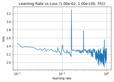
We first ran the LRFinder for a relatively large learning rate range from 1e-6 to 3. This gives us the chart on the left below. For the CLR schedule, the minimum LR for our range is where the loss starts descending, and the maximum LR is where the loss stops descending or becomes ragged. My charts are not as clean as those shown in the two projects referenced, but we can still infer that these boundaries are 1e-6 and about 3e-1. The chart on the right below is the plot of LR vs Loss on a smaller range (1e-2 and 1) to help see the chart in greater detail. We also see that the LR with minimum loss is about 3e-1.


Based on this, my first experiment is to try and train the network with the larger best learning rate (3e-1) we found from the LR Finder, and see if it trains better over 10 epochs than my previous attempt. The only thing we have changed here from the previous training code block above is to replace learning_rate from 0.001 to 0.3. Here are the results of 10 epochs of training, followed by evaluation on the held out test set.

Epoch 1/10
351/351 [==============================] - 12s 36ms/step - loss: 2.1572 - accuracy: 0.1664 - val_loss: 1.9966 - val_accuracy: 0.2590
Epoch 2/10
351/351 [==============================] - 12s 34ms/step - loss: 1.8960 - accuracy: 0.2979 - val_loss: 1.7568 - val_accuracy: 0.3732
Epoch 3/10
351/351 [==============================] - 12s 35ms/step - loss: 1.7456 - accuracy: 0.3642 - val_loss: 1.6556 - val_accuracy: 0.3984
Epoch 4/10
351/351 [==============================] - 12s 35ms/step - loss: 1.6634 - accuracy: 0.4021 - val_loss: 1.6050 - val_accuracy: 0.4331
Epoch 5/10
351/351 [==============================] - 12s 35ms/step - loss: 1.5993 - accuracy: 0.4213 - val_loss: 1.6906 - val_accuracy: 0.3858
Epoch 6/10
351/351 [==============================] - 12s 36ms/step - loss: 1.5244 - accuracy: 0.4484 - val_loss: 1.5754 - val_accuracy: 0.4399
Epoch 7/10
351/351 [==============================] - 13s 36ms/step - loss: 1.4568 - accuracy: 0.4749 - val_loss: 1.4996 - val_accuracy: 0.4712
Epoch 8/10
351/351 [==============================] - 13s 36ms/step - loss: 1.3894 - accuracy: 0.4971 - val_loss: 1.4854 - val_accuracy: 0.4786
Epoch 9/10
351/351 [==============================] - 12s 35ms/step - loss: 1.3323 - accuracy: 0.5207 - val_loss: 1.4527 - val_accuracy: 0.4950
Epoch 10/10
351/351 [==============================] - 12s 36ms/step - loss: 1.2817 - accuracy: 0.5411 - val_loss: 1.4320 - val_accuracy: 0.5068

78/78 [==============================] - 1s 12ms/step - loss: 1.4477 - accuracy: 0.4920

Clearly, the larger learning rate is helping the network achieve better performance, although it does seem (at least around epoch 3) that it may be slightly too large. Accuracy numbers on the held out test set jumped from 0.3112 to 0.4920. So overall it seems to be helping. So even if we just use the LR Finder to find the "best" learning rate, this is still cheaper than doing multiple training runs of a few epochs each.

Finally, we will try using a Cyclic Learning Rate (CLR) schedule using the learning rate boundaries (1e-6, 3e-1). The code for this is shown below. The clr_schedule() function produces a triangular learning rate schedule which rises for the first 5 epochs (in our case) from the minimum specified learning rate to the maximum, then falls from the maximum to the minimum for the next 4 epochs, and finally falls to half the minimum for the last epoch. This is analogous to the Learner.fit_one_cycle() call in fast.ai. The clr_schedule function is passed to the LearningRateScheduler callback, which is then called by the model training loop via the callback parameter in the fit() function call. Here is the code.

1 2 3 4 5 6 7 8 9 10 11 12 13 14 15 16 17 18 19 20 21 22 23 24 25 26 27 28 29 30 31 32 33 34 35 36 37 38

import matplotlib.pyplot as plt import numpy as np import tensorflow as tf def clr_schedule(epoch): num_epochs = 10 mid_pt = int(num_epochs * 0.5) last_pt = int(num_epochs * 0.9) min_lr, max_lr = 1e-6, 3e-1 if epoch <= mid_pt: return min_lr + epoch * (max_lr - min_lr) / mid_pt elif epoch > mid_pt and epoch <= last_pt: return max_lr - ((epoch - mid_pt) * (max_lr - min_lr)) / mid_pt else: return min_lr / 2 # plot the points # epochs = [x+1 for x in np.arange(10)] # clrs = [clr_schedule(x) for x in epochs] # plt.plot(epochs, clrs) # plt.show() batch_size = 128 train_dataset, val_dataset, test_dataset = load_cifar10_data(batch_size) model = LeNetModel() min_lr = 1e-6 max_lr = 3e-1 optimizer = tf.keras.optimizers.SGD(learning_rate=min_lr) loss_fn = tf.keras.losses.CategoricalCrossentropy() lr_scheduler = tf.keras.callbacks.LearningRateScheduler(clr_schedule) model.compile(loss=loss_fn, optimizer=optimizer, metrics=["accuracy"]) model.fit(train_dataset, epochs=10, validation_data=val_dataset, callbacks=[lr_scheduler]) model.evaluate(test_dataset)

And here are the results of training the LeNet model with the CIFAR-10 dataset for 10 epochs, and evaluating on the held out test set. As you can see, the evaluation accuracy on the held out test set has jumped further from 0.4920 to 0.5469.

Epoch 1/10
351/351 [==============================] - 13s 36ms/step - loss: 2.7753 - accuracy: 0.0993 - val_loss: 2.7627 - val_accuracy: 0.1060
Epoch 2/10
351/351 [==============================] - 12s 34ms/step - loss: 2.0131 - accuracy: 0.2097 - val_loss: 2.0829 - val_accuracy: 0.2634
Epoch 3/10
351/351 [==============================] - 12s 34ms/step - loss: 1.8321 - accuracy: 0.3106 - val_loss: 1.7187 - val_accuracy: 0.3718
Epoch 4/10
351/351 [==============================] - 12s 35ms/step - loss: 1.7100 - accuracy: 0.3648 - val_loss: 1.7484 - val_accuracy: 0.3928
Epoch 5/10
351/351 [==============================] - 12s 36ms/step - loss: 1.5779 - accuracy: 0.4209 - val_loss: 1.6188 - val_accuracy: 0.4087
Epoch 6/10
351/351 [==============================] - 13s 36ms/step - loss: 1.5451 - accuracy: 0.4300 - val_loss: 1.5704 - val_accuracy: 0.4377
Epoch 7/10
351/351 [==============================] - 12s 35ms/step - loss: 1.3597 - accuracy: 0.5063 - val_loss: 1.3742 - val_accuracy: 0.5014
Epoch 8/10
351/351 [==============================] - 12s 36ms/step - loss: 1.2383 - accuracy: 0.5484 - val_loss: 1.3620 - val_accuracy: 0.5204
Epoch 9/10
351/351 [==============================] - 12s 35ms/step - loss: 1.1379 - accuracy: 0.5856 - val_loss: 1.3336 - val_accuracy: 0.5391
Epoch 10/10
351/351 [==============================] - 12s 35ms/step - loss: 1.0564 - accuracy: 0.6130 - val_loss: 1.3008 - val_accuracy: 0.5557

78/78 [==============================] - 1s 13ms/step - loss: 1.3043 - accuracy: 0.5469

This indicates that the LR Finder and CLR schedule seem like good ideas to try when training your models, especially when using non-adaptive optimizers such as SGD.

I tried the same sequence of experiments with the Adam optimizer, and I got better results (test accuracy: 0.5908) using a fixed learning rate of 1e-3 for the first training run. Thereafter, based on the LR Finder reporting a learning rate range of (1e-6, 1e-1), the next two experiments using the best learning rate and CLR schedule both produced accuracies of about 0.1 (i.e., close to random for 10-class classifier). I wasn't too surprised, since I figured that the CLR schedule probably interfered with Adam's own learning rate schedule. However, according to this tweet from Jeremy Howard, the LR Finder can be used with the Adam optimizer as well. Given that he has probably conducted many more experiments around this than I have, and the fast.ai Learner.lr_find() code is more robust and heavily tested than my homegrown implementation, he is very likely right, and my results are an anomaly.

That's all I have for today. Thanks for staying with me so far. I learned a lot from implementing this code, and hopefully you learned a few things from reading this as well. Hopefully, this gives you some ideas for building an LR Finder for Tensorflow 2 that can be used easily by end-users -- if you do end up building one, please let me know, will be happy to link to your site/repository and recommend it to other readers.

AWS ML Week and adventures with SageMaker

I attended the AWS ML Week at San Francisco couple of weeks ago. It was held over 2 days and consisted of presentations and workshops, presented and run by Amazon Web Services (AWS) architects. The event was meant to showcase the ML capabilities of AWS and was targeted at Data Scientists and Engineers, as well as innovators who want to include Machine Learning (ML) capabilities in their applications.

The AWS ML stack at the time of writing is as shown below. This image comes from one of the presentation slides. The top layer (Application Services) is a set of canned ML models exposed through an API and is aimed at people who want to exploit ML capabilities in their applications without having to go through the hassle of building it themselves. The middle layer (Platform Services) is aimed at the Data Scientist / Engineer types who are training and consuming their own ML models. The bottom layer (Frameworks and Interfaces) is the infrastructure layer, based upon the Amazon Deep Learning AMIs that were released some time back.

The first day of talks covered the Application Services (top) layer, and the second day covered the Platform Services (middle) layer. The Frameworks and Interfaces (bottom) layer was not covered at all, but those of us who've trained Deep Learning (DL) models on AWS have probably used the Amazon Deep Learning AMIs and know enough about them already.

My main reason for attending the event was twofold. First, some colleagues were talking about the cool canned ML algorithms that AWS was coming out with, and I thought attending this kind of event would be a way to quickly learn about them all at a high level. Second, a colleague and I had evaluated SageMaker earlier for our own use, and I had concluded that while it was a good managed notebook environment for development, I wasn't too impressed with its stated goal as an unified platform for distributed model training and deployment, and I was hoping that I would learn new information here that would change my mind.

In this post, I will focus on these two aspects in depth.

Application Services

This is just a list of application services with a brief description. All of these can be consumed through an API, and provide very general services such as emotion detection in faces, keyword extraction from text, etc. However, it is often possible to compose these undifferentiated services to produce unique functionality. Such applications can just use the AWS Application Services rather than build them themselves, saving them some time and wheel reinvention effort in the process.

• Rekognition - a group of Computer Vision (CV) services. There is a Rekognition for Images and a Rekognition for Video. Rekognition for Images provides functionality for Object and Scene Detection, Facial Analysis (sentiment, gender, facial features), Face Recognition, Unsafe (NSFW) detection, Celebrity recognition, Text in Images and Face Similarity comparison. Rekognition for Video has all the services of Rekognition for Images plus Person tracking.
• Transcribe - speech to text conversion. This was in preview at the time but has since become generally available. Unlike other services, the API is asynchronous only.
• Translate - language translation. Supported only English and Spanish at the time, but they are adding more languages, so this might have changed also. As with Transcribe, it was in preview but has become generally available.
• Comprehend - a set of language services that work on text to detect sentiment, entities, language and key phrases. It also has functionality to build topic models out of a corpus of text.
• Polly - text to speech conversion. Multiple voices and accents available for customization.
• Lex - conversational interface for text and voice based applications, it is the API underlying the Amazon Echo and Alexa family of devices.

Some examples of applications that could be composed using these components are listed below. Some of these are covered in more depth in the presentation slides (see list at bottom).

• Using Comprehend to detect non-English tweets and translate to translate them into English, and extract keywords from them using Comprehend.
• Using Comprehend to generate sentiment on incoming customer service requests.
• Extracting entities and keyphrases from a text corpus to generate knowledge graphs.
• Video captioning of different languages simultaneously using Translate.
• Pollexy project (video) - application to remind autistic child to do specific things at different times of the day.
• Finding missing persons by comparing images on social media with reference image - this was our workshop example from day 1.

SageMaker

SageMaker bills itself as a fully-managed platform to build, train and deploy ML models at scale. As a user, I see two main use cases - a managed notebook platform for development, and a unified platform for training and deploying ML models.

For the first use case, as long as you are using Keras, Tensorflow (TF) or MXNet with either Python2 or Python3, you could simply choose the appropriate notebook type and use it. You could also install other frameworks such as Pytorch using pip on the notebook's virtual terminal and use that instead. It's not very different from running Jupyter notebooks on your Deep Learning AMI and possibly a little less flexible, but it can be convenient for enterprise customers with their own Virtual Private Clouds (VPCs) since the SageMaker notebook is available within your Amazon console without having to do complex network finagling. Strangely enough, Amazon does not emphasize this use case at all.

The other use case is as a unified platform for large scale (possibly distributed) model training and model deployment. In this mode, SageMaker acts as a wrapper that calls into user provided functionality at different points in its life cycle. This allows you to run the SageMaker notebook on a relatively low end EC2 instance because you would spin up a high performance EC2 box (possibly even a GPU box if needed) for the duration of the training. Similarly, you would deploy the trained model to a different EC2 instance as well. In Java object oriented terms, SageMaker does this by exposing an Estimator interface that various ML models must implement. In this mode, SageMaker supports a wide variety of ML algorithms (Deep Learning and traditional), as listed below.

• Built-in ML algorithms - the following algorithms are provided as part of SageMaker - Linear Learner, Factorization Machines, XGBoost, Image Classification, Sequence2Sequence, KMeans, Principal Components Analysis (PCA), Latent Dirichlet Allocation (LDA), Neural Topic Models (NTM), DeepAR Forecasting (Time Series) and BlazingText (word2vec implementation). The built-in algorithms are all exposed via a common Estimator interface that uses Docker registry paths to identify a specific algorithm.
• MXNet and TF Estimators - these SageMaker Estimators allow wrapping of the user's MXNet and TF models (as well as Keras models built using Keras embedded in TF, also known as tf.keras). The user has to provide implementations of certain functions to SageMaker and SageMaker calls them at different points in its lifecycle. Since TF comes with its own Estimators which are pre-built DL and ML networks, this opens up even more possibilities. So overall, this allows wrapping of the following kinds of models.
  
  • MXNet models (including prebuilt models from around the net and from the MXNet model zoo)
  • TF Estimators (list of pre-made Estimators from TF docs)
  • TF models (including prebuilt models from around the net and from the recently announced Tensorflow Hub)
  • Keras models (including prebuilt models from around the net and from the Keras model zoo)
• Bring Your Own Model (BYOM) Estimators - you set up a Docker contiainer in a specific way to expose training and serving functionality via scripts, and the SageMaker Estimator would use these scripts to train and deploy the model. This is the same Estimator that exposes SageMaker's built-in ML functionality.

Examples of each of these use cases can be found in the awslabs/amazon-sagemaker-examples repository. We did run through some of these in one of the workshops, but I decided to expose one of my own recent Keras models through SageMaker to figure out the steps involved.

The documentation about wrapping TF/Keras models on the aws/sagemaker-python-sdk repository says that the training script must contain the following function overrides.

• Exactly one of model_fn, keras_model_fn or estimator_fn - defines the model to be trained, each of the options correspond to definitions for one of TF model, tf.keras model or TF Estimator respectively
• train_input_fn - to preprocess and load training data
• eval_input_fn - to preprocess and load evaluation data
• serving_input_fn - required for deploying endpoint through SageMaker

My model takes as input dense vectors of size (2048,) and predicts one of two classes. Since the model was built using tf.keras I started by defining a keras_model_fn and the other function overrides as follows:

1 2 3 4 5 6 7 8 9 10 11 12 13 14 15 16 17 18 19 20 21 22 23 24 25 26 27 28 29 30 31 32 33 34 35 36 37 38 39 40 41 42 43 44 45 46 47 48 49 50 51 52 53 54 55 56 57 58 59 60 61 62 63 64 65 66 67

import boto3 import numpy as np import os import tensorflow as tf from tensorflow.python.estimator.export.export import build_raw_serving_input_receiver_fn INPUT_TENSOR_NAME = 'inputs_input' # needs to match the name of the first layer + "_input" hyperparams = { "learning_rate": 1e-3 } def keras_model_fn(hyperparams): # build model model = tf.keras.models.Sequential() model.add(tf.keras.layers.Dense(2048, input_shape=(2048,), name="inputs")) model.add(tf.keras.layers.Activation("relu")) model.add(tf.keras.layers.Dropout(0.5)) model.add(tf.keras.layers.Dense(512)) model.add(tf.keras.layers.Activation("relu")) model.add(tf.keras.layers.Dropout(0.5)) model.add(tf.keras.layers.Dense(128)) model.add(tf.keras.layers.Activation("relu")) model.add(tf.keras.layers.Dropout(0.5)) model.add(tf.keras.layers.Dense(2)) model.add(tf.keras.layers.Activation("softmax", name="output")) # compile model optim = tf.keras.optimizers.Adam(lr=hyperparams["learning_rate"]) model.compile(optimizer=optim, loss="categorical_crossentropy", metrics=["accuracy"]) return model def train_input_fn(training_dir, hyperparams): return _train_eval_input_fn(training_dir, "train_file.csv") def eval_input_fn(training_dir, hyperparams): return _train_eval_input_fn(training_dir, "eval_file.csv") def _train_eval_input_fn(training_dir, training_file): xs, ys = [], [] ftest = open(os.path.join(training_dir, training_file), "rb") for line in ftest: _, label, vec_str = line.strip().split("\t") xs.append(np.array([float(e) for e in vec_str.split(",")])) ys.append(int(label)) ftest.close() X = np.array(xs, dtype=np.float32) Y = tf.keras.utils.to_categorical( np.array(ys), num_classes=2).astype(np.int) return tf.estimator.inputs.numpy_input_fn( x={INPUT_TENSOR_NAME: X}, y=Y, num_epochs=None, shuffle=True)() def serving_input_fn(hyperparams): tensor = tf.placeholder(tf.float32, [1, 2048]) return build_raw_serving_input_receiver_fn({INPUT_TENSOR_NAME: tensor})()

Later, however, I found that the deployed model was not able to parse request vectors serialized by TF's make_proto mechanism, so I had to switch to treating it as a TF model instead. This just meant that I had to replace the keras_model_fn with a model_fn function. The other change was that now my INPUT_TENSOR_NAME was no longer under the control of the Keras API, so I could rename it to the more readable "inputs". In addition, since I now have to explicitly provide EstimatorSpec objects for each of my operation modes (train, eval, predict), I need an additional import (PredictOutput) and an additional prediction signature key given by SIGNATURE_NAME. Also notice how the model definition has changed from the Sequential model to a functional form, where the input to the network comes from the features parameter. The other functions remain unchanged.

1 2 3 4 5 6 7 8 9 10 11 12 13 14 15 16 17 18 19 20 21 22 23 24 25 26 27 28 29 30 31 32 33 34 35 36 37 38 39 40 41 42 43 44 45 46 47

from tensorflow.python.estimator.export.export_output import PredictOutput INPUT_TENSOR_NAME = "inputs" SIGNATURE_NAME = "serving_default" def model_fn(features, labels, mode, hyperparams): # build model (notice no input layer, fed from features parameter) hidden_1 = tf.keras.layers.Dense(2048, activation="relu")(features[INPUT_TENSOR_NAME]) hidden_1 = tf.keras.layers.Dropout(0.5)(hidden_1) hidden_2 = tf.keras.layers.Dense(512, activation="relu")(hidden_1) hidden_2 = tf.keras.layers.Dropout(0.5)(hidden_2) hidden_3 = tf.keras.layers.Dense(128, activation="relu")(hidden_2) hidden_3 = tf.keras.layers.Dropout(0.5)(hidden_3) predictions = tf.keras.layers.Dense(2, activation="softmax", name="output")(hidden_3) # estimator for predictions if mode == tf.estimator.ModeKeys.PREDICT: return tf.estimator.EstimatorSpec( mode=mode, predictions={"output": predictions}, export_outputs={SIGNATURE_NAME: PredictOutput({"output": predictions})}) # define loss function (using TF) loss = tf.losses.softmax_cross_entropy(labels, predictions) # define training op (using TF) train_op = tf.contrib.layers.optimize_loss( loss=loss, global_step=tf.train.get_global_step(), learning_rate=hyperparams["learning_rate"], optimizer="Adam") # generate predictions as TF tensors predictions_dict = {"output": predictions} # generate eval_metric ops eval_metric_ops = { "accuracy": tf.metrics.accuracy( tf.cast(labels, tf.float32), predictions) } # estimator for train and eval return tf.estimator.EstimatorSpec( mode=mode, loss=loss, train_op=train_op, eval_metric_ops=eval_metric_ops)

The above functions are written out into a script file and passed into the SageMaker Estimator. I tested each individual function separately to verify that they work by themselves. I did note that the SageMaker Estimator code (as well as TF code) is much more picky about data types - for the features, it expects a matrix of np.float32 and for the labels it expects a vector of np.int. Here is the code to train this model using SageMaker.

1 2 3 4 5 6 7 8 9 10 11 12 13 14 15 16 17 18 19 20 21 22 23 24 25 26 27 28 29 30 31 32 33 34 35 36 37 38 39 40 41 42 43 44 45 46

import json import numpy as np import os import sagemaker import tensorflow as tf from sagemaker import get_execution_role from sagemaker.tensorflow import TensorFlow # (1) set up sagemaker_session = sagemaker.Session() # role = get_execution_role() role = "arn:aws:iam:..." # copy-paste the IAM role from your SageMaker console # (2) upload data to S3 inputs = sagemaker_session.upload_data(path="data/", key_prefix="data") # (3) train model compdetect_estimator = TensorFlow(entry_point="composite-detector-tf.py", role=role, training_steps=100, evaluation_steps=100, hyperparameters={"learning_rate": 1e-3}, train_instance_count=1, train_instance_type="ml.p2.xlarge") compdetect_estimator.fit(inputs) # (4) deploy model compdetect_predictor = compdetect_estimator.deploy(initial_instance_count=1, instance_type='ml.m4.xlarge') # (5) load data for evaluation and run predictions Xeval = load_eval_data() for i in range(Xeval.shape[0]): data = Xeval[i] tensor_proto = tf.make_tensor_proto(values=np.asarray(data), shape=[1, len(data)], dtype=tf.float32) pred = compdetect_predictor.predict(tensor_proto) Y_ = pred["outputs"]["output"]["floatVal"] y = np.argmax(Y_) print(i, y) # (6) delete the endpoint when done sagemaker.Session().delete_endpoint(compdetect_predictor.endpoint)

Below I explain each of these steps in detail.

1. The first step is to open a SageMaker session and extract the IAM role from it. There seems to be a bug in this code, so I found (and others on the Internet have the same advice) that just using the IAM role value from the SageMaker notbook console works just as well.
2. Lately, I usually have code in my notebooks to copy any data I need (and don't already have locally) from S3 and write back my models and output datasets back to S3 using the boto3 package. Here, the upload_data call expects to see the data locally, so I used awscli to copy it down from S3 to a local data subfolder, then invoke the command. The upload_data command will place it in a well-known (within the session) S3 bucket accessible to the training instance as well.
3. The next step is to train the model. The entry_point parameter to the Tensorflow Estimator points to the script file with the functions that we set up above. The only hyperparameter we are passing in is the learning rate. The training will be done on a single m1.p2.xlarge instance (as indicated by the train_instance_count and train_instance_type parameters). We could have used distributed training by setting the train_instance_count to a value larger than 1. Note that tf.keras models exposed through the keras_model_fn cannot be trained in distributed mode. The model trains for 100 iterations and is evaluated for 100 iterations.
4. Once trained, the model is deployed to yet another m1.m4.xlarge instance, called the endpoint, with the estimator.deploy call. The endpoint can auto-scale, meaning that SageMaker can automatically spin up additional instances of the endpoint in case the usage goes too high.
5. We can now run predictions against the model by hitting the endpoint. Our endpoint is set up to consume input one at a time, but we could also set it up to consume fixed size batches if desired. The data has to be serialized using tf.make_tensor_proto and then passed to the predictor.predict call. This was the part that was failing for my Estimator using the keras_model_fn function, I suspect it has to do mismatch between the way TF serializes the data and the way Keras expects it. A sample output from the endpoint is shown below.
   
   
   
6. Finally, if we no longer need to use the endpoint, we can just destroy it using delete_endpoint call. We can also delete it from the console.

So that's what it took to wrap my model into a SageMaker estimator and train and deploy it. Its not a lot of code, but documentation and Stack Overflow style support is still scarce, so the going is not very smooth. However, having trained and deployed one network through SageMaker, I feel more confident of being able to do the same with others. So given that it's a pain to work with, but does provide a lot of benefits, I have reconsidered my original skepticism towards it.

Other stuff: IoT and DeepLens

The last two talks focused on ML on IoT devices using MXNet. Models could be on-board on the IoT device or be accessed from the cloud over a SageMaker endpoint or using AWS Greengrass. In line with the focus on IoT, AWS DeepLens device is a device that can host ML algorithms, either canned ones from the AWS ML Application Services layer, or those you build yourself. Similar to the Echo/Alexa family of devices, I think DeepLens is meant to catalyze development of novel ML and CV applications for the consumer market. It is expected to be available in June 2018 and is available for pre-order on Amazon.

Links to Slides

Links to presentation slides were provided after the event and are all publicly available on Slideshare, would be awesome (wink wink nudge nudge, AWS guys) if these links were also updated on the original event page for AWS ML Week.

• Day 1 (Monday, March 26 2018)
  
  • Build Intelligent Applications with AWS ML Services - by Steve Shirkey, Solutions Architect, AWS
  • Automate for Efficiency with Amazon Transcribe and Amazon Translate - by Niranjan Hira, Solutions Architect, AWS
  • Using Amazon Comprehend and Amazon SageMaker to gain insights from text - by Nino Bice, Sr Product Manager, AWS
  • Build a Virtual Assistant with Amazon Polly and Amazon Lex (workshop) - by Niranjan Hira, Solutions Architect, AWS
  • Using Amazon Rekognition to build a Facial Recognition System (workshop) - by Kashif Imran, Solutions Architect, AWS
• Day 2 (Tuesday, March 27 2018)
  
  • Using Amazon SageMaker to build, train and deploy your ML Models - by Gitansh Chadha, Solutions Architect, AWS
  • SageMaker Algorithms: Infinitely Scalable Machine Learning - by Amit Sharma, Principal Solutions Architec, AWS
  • Integrating Deep Learning into your Enterprise - by Yash Pant, Enterprise Solutions Architect, AWS
  • Building Deep Learning Applications with Tensorflow and Amazon SageMaker (workshop) - by Steve Shirkey, Solutions Architect, AWS
  • Enabling Deep Learning in IoT Applications with Apache MXNet - by Pratap Ramamurthy, Partner Solutions Architec and Hagay Lupesco, Software Development Engineer, AWS
  • AWS DeepLens: A new way to learn Machine Learning - by Mike Miller, Sr Manager, AWS

So that's all I had for the AWS ML Week. I think I ended up getting what I went there for. First I now have a good idea of the different services available in the Application Services layer. Second, I have a much better understanding and appreciation of SageMaker. I hope you found my writeup useful as well.