Disambiguating SciSpacy + UMLS entities using the Viterbi algorithm

The SciSpacy project from AllenAI provides a language model trained on biomedical text, which can be used for Named Entity Recognition (NER) of biomedical entities using the standard SpaCy API. Unlike the entities found using SpaCy's language models (at least the English one), where entities have types such as PER, GEO, ORG, etc., SciSpacy entities have the single type ENTITY. In order to further classify them, SciSpacy provides Entity Linking (NEL) functionality through its integration with various ontology providers, such as the Unified Medical Language System (UMLS), Medical Subject Headings (MeSH), RxNorm, Gene Ontology (GO), and Human Phenotype Ontology (HPO). 

The NER and NEL processes are decoupled. The NER process finds candidate entity spans, and these spans are matched against the respective ontologies, which may result in the span matching zero or more ontology entries. All candidate span is then matched to all the matched entities. 

I tried annotating the COVID-19 Open Research Dataset (CORD-19) against UMLS using the SciSpacy integration described above, and I noticed significant ambiguity in the linking results. Specifically, annotating approximately 22 million sentences in the CORD-19 dataset results in 113 million candidate entity spans, which get linked to 166 million UMLS concepts, i.e., on average, each candidate span resolves to 1.5 UMLS concepts. However, the distribution is Zipfian, with approximately 46.87% entity spans resolving to a single concept, with a long tail of entity spans being linked to up to 67 UMLS concepts. 

In this post, I will describe a strategy to disambiguate the linked entities. Based on limited testing, this chooses the correct concept about 73% of the time. 

The strategy is based on the intuition that an ambiguously linked entity span is more likely to resolve to a concept that is closely related to concepts for the other non-ambiguously linked entity spans in the sentence. In other words, the best target label to choose for an ambiguous entity is the one that is semantically closest to the labels of other entities in the sentence. Or even more succintly, and with apologies to John Firth, an entity is known by the company it keeps. 

The NER and NEL processes provided by the SciSpacy library allows us to reduce a sentence to a collection of entity spans, each of which map to zero or more UMLS concepts. Each UMLS concept maps to one or more Semantic Types, which represent high level subject categories. So essentially, a sentence can be reduced to a graph of semantic type using the following steps. 

Consider the sentence below, the NER step identifies candidate spans that are indicated by highlights.

The fact that viral antigens could not be demonstrated with the used staining is not the result of antibodies present in the cat that already bound to these antigens and hinder binding of other antibodies.

The NEL step will attempt to match these spans against the UMLS ontology. Results for the matching are shown below. As noted earlier, each UMLS concept maps to one or more sematic types, and these are shown here as well.

   

Entity-ID	Entity Span	Concept-ID	Concept Primary Name	Semantic Type Code	Semantic Type Name
1	staining	C0487602	Staining method	T059	Laboratory Procedure
2	antibodies	C0003241	Antibodies	T116	Amino Acid, Peptide, or Protein
				T129	Immunologic Factor
3	cat	C0007450	Felis catus	T015	Mammal
		C0008169	Chloramphenicol O-Acetyltransferase	T116	Amino Acid, Peptide, or Protein
				T126	Enzyme
		C0325089	Family Felidae	T015	Mammal
		C1366498	Chloramphenicol Acetyl Transferase Gene	T028	Gene or Genome
4	antigens	C0003320	Antigens	T129	Immunologic Factor
5	binding	C1145667	Binding action	T052	Activity
		C1167622	Binding (Molecular Function)	T044	Molecular Function
6	antibodies	C0003241	Antibodies	T116	Amino Acid, Peptide, or Protein
				T129	Immunologic Factor

The sequence of entity spans, each mapped to one or more semantic type codes can be represented by a graph of semantic type nodes as shown below. Here, each vertical grouping corresponds to an entity position. The BOS node is a special node representing the beginning of the sequence. Based on our intuition above, entity disambiguation is now just a matter of finding the most likely path through the graph.

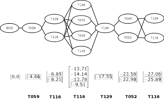
Of course, "most likely" implies that we need to know the probabilities for transitioning between semantic types. We can think of the graph as a Markov Chain, and consider the probability of each node in the graph as being determined only by its previous node. Fortunately, this information is already available as a result of the NER + NEL process for the entire CORD-19 dataset, where approximately half of the entity spans mapped unambiguously to a single UMLS concept. Most concepts map to a single semantic type, but in cases where they map to multiple, we consider them as separate records. We compute pairwise transition probabilities across semantic types for these unambiguously linked pairs across the CORD-19 dataset and create our transition matrix. In addition, we also create a matrix of emission probabilities that identify the probabilities of resolving to a concept given a semantic type. 

Using the transition probabilities, we can traverse each path in the graph from starting to ending position, computing the path probability as the product of transition probabilities (or for computational reasons, the sum of log-probabilities) of the edges. However, better methods exist, such as the Viterbi algorithm, which allows us to save on repeated computation of common edge sequences across multiple paths. This is what we used to compute the most likely path through our semantic type graph. 

The Viterbi algorithm consists of two phases -- forward and backward. In the forward phase, we move left to right, computing the log-probability of each transition at each step, as shown by the vectors below each position in the figure. When computing the transition from multiple nodes to a single node (such as the one from [T129, T116] to [T126], we compute for both paths and choose the maximum value. 

In the backward phase, we move from right to left, choosing the maximum probability node at each step. This is shown in the figure as boxed entries. We can then lookup the appropriate semantic type and return the most likely sequence of semantic types (shown in bold in the bottom of the figure). 

However, our objective is to return disambiguated concept linkages for entities. Given a disambiguated semantic type and multiple possibilities indicated by SciSpacy's linking process, we use the emission probabilities to choose the most likely concept to apply at the position. The result for our example is shown in the table below.

Entity-ID	Entity Span	Concept-ID	Concept Primary Name	Semantic Type Code	Semantic Type Name	Correct?
1	staining	C0487602	Staining method	T059	Laboratory Procedure	N/A*
2	antibodies	C0003241	Antibodies	T116	Amino Acid, Peptide, or Protein	Yes
3	cat	C0008169	Chloramphenicol O-Acetyltransferase	T116	Amino Acid, Peptide, or Protein	No
4	antigens	C0003320	Antigens	T129	Immunologic Factor	N/A*
5	binding	C1145667	Binding action	T052	Activity	Yes
6	antibodies	C0003241	Antibodies	T116	Amino Acid, Peptide, or Protein	Yes

(N/A: non-ambiguous mappings) 

I thought this might be an interesting technique to share, hence writing about it. In addition, in the spirit of reproducibility, I have also provided the following artifacts for your convenience.

1. Code: This github gist contains code that illustrates NER + NEL on an input sentence using SciSpacy and its UMLS integration, and then applies my adaptation of the Viterbi method (as described in this post) to disambiguate ambiguous entity linkages.
2. Data: I have also provided the transition and emission matrices, and their associated lookup tables, for convenience, as these can be time consuming to generate from scratch from the CORD-19 dataset.

As always, I appreciate your feedback. Please let me know if you find flaws with my approach, and/or you know of a better approach for entity disambiguation

Counting Triangles in a Movie Actor Network

I recently came across an algorithm to list all triangles in a graph in the Data Algorithms book. I didn't have a real application to use it against, but given that counting triangles have quite a few uses, I figured it would be useful to try and implement in Spark. So thats what this post is all about.

The algorithm is somewhat non-trivial, so I will use the very simple graph shown below to explain the algorithm step-by-step. You can instantly see that the two triangles in this graph are (2, 3, 4) and (2, 4, 5). Here is the Spark code that implements the algorithm.

1 2 3 4 5 6 7 8 9 10 11 12 13 14 15 16 17 18 19 20 21 22 23 24 25 26 27 28 29 30 31 32 33 34 35 36 37 38 39 40

def addReverseEdge(pair: (Long, Long)): List[(Long, Long)] = { val reverse = (pair._2, pair._1) List(pair, reverse) } def buildEdges(u: Long, vs: List[Long]): List[((Long, Long), Long)] = { val uvpairs = vs.map(v => ((u, v), -1L)) val vpairs = for (v1 <- vs; v2 <- vs) yield ((v1, v2), u) uvpairs ++ vpairs.filter(vv => vv._1._1 < vv._1._2) } def buildTriangles(uv: (Long, Long), ws: List[Long]): List[((Long, Long, Long), Int)] = { val hasAnchor = ws.filter(_ < 0).size > 0 val onlyAnchor = ws.size == 1 && hasAnchor if (hasAnchor && !onlyAnchor) { ws.filter(w => w > 0) .map(w => { val nodes = List(uv._1, uv._2, w).sorted ((nodes(0), nodes(1), nodes(2)), 1) }) } else List.empty } // val actorPairs = sc.parallelize(List( // (1L, 2L), (2L, 3L), (2L, 4L), (2L, 5L), (3L, 4L), (4L, 5L))) val actorPairs = sc.textFile("/path/to/actor_pairs.tsv") .map(line => line.split('\t')) .map(cols => (cols(0).toLong, cols(1).toLong)) .cache val triangles = actorPairs.flatMap(kv => addReverseEdge(kv)) // (u, v) += (v, u) .map(kv => (kv._1, List(kv._2))) // (u, [v]) .reduceByKey((a, b) => a ++ b) // (u, [v1, v2, ...]) .flatMap(kvs => buildEdges(kvs._1, kvs._2)) // ((u, v), w) .mapValues(w => List(w)) // ((u, v), [w]) .reduceByKey((a, b) => a ++ b) // ((u, v), [w1, w2, ...]) .flatMap(uvws => buildTriangles(uvws._1, uvws._2)) // ((u, v, w), 1) .reduceByKey((a, b) => a + b) // ((u, v, w), count) - dedup triangles .cache

Input to the algorithm is a list of edges, each edge being represented as a pair of vertex IDs. We ensure that each edge is represented exactly once by ensuring that the source vertex ID is less than the target vertex ID. For our graph, the input looks like this:

1	(1, 2), (2, 3), (2, 4), (2, 5), (3, 4), (4, 5)

The first flatMap call on actorPairs adds a reverse edge, ie, for every (u, v) edge we add an additional (v, u) edge. We do this because we will use the LHS vertex to group on, considering each vertex as the start vertex for our triangles. Once we are done, our data looks like this:

1	(1, [2]), (2, [3, 1, 4, 5]), (3, [2, 4]), (4, [3, 2, 5]), (5, [2, 4])

The next three lines build up edges with our left vertex and each vertex on the list on the right hand element of each pair, then group the third vertex by the edge. The result of this operation looks like this:

1 2 3

((4, 2), [-1]), ((3, 4), [-1, 2]), ((1, 4), [2]), ((2, 3), [-1, 4]), ((5, 4), [-1]), ((1, 2), [-1]), ((5, 2), [-1]), ((3, 5), [2, 4]), ((2, 5), [-1, 4]), ((1, 3), [2])

The next line groups by all three edges and removes any invalid vertex triples. Since a triangle can be created in one of 3 ways using a set of three vertices, we want to dedup this by sorting the vertex IDs. The step returns the sorted vertex set and a 1, and the next line counts the vertex set representing the triangle.

1	((2, 3, 4), 3), ((2, 4, 5), 3)

For my data, I used the list of movies, actors and actresses, available as plain text files from the IMDB Dataset. The dataset contains 3.6 million movies and TV shows, 2.2 million actors and 1.2 million actresses. The formats are as follows:

1 2 3 4 5 6 7 8 9 10 11 12 13 14 15 16 17 18

# movies.list # movie-name \t release-year Star Wars VII: Return of the Empire (2013) 2013 ... # actors.list # actor-name \t movie-name [role] # \t \t movie-name [role] Carl, Shay Bro-Friend (2012) [Brother] Star Wars VII: Return of the Empire (2013) [Obi Wan] ... # actresses.list # actress-name \t movie-name [role] # \t \t movie-name [role] Katz, Liz 2 Big 2 Be True 8 (2007) (V) [(as Risi Simms)] Star Wars VII: Return of the Empire (2013) [Princess Leia] ...

In order to get this data into the vertex-pair format we need, we used the following Python code to do the conversion. Since we were only interested in movies, we skipped all TV shows listed (names beginning with quotes). We first created actor-movie pairs (out of both actor and actress files), then grouped on movies to find all actors that worked together in the movie, and then built edges out of these actors.

1 2 3 4 5 6 7 8 9 10 11 12 13 14 15 16 17 18 19 20 21 22 23 24 25 26 27 28 29 30 31 32 33 34 35 36 37 38 39 40 41 42 43 44 45 46 47 48 49 50 51 52 53 54 55 56 57 58 59 60 61 62 63 64 65 66 67 68 69 70 71 72 73 74 75 76 77 78 79 80 81 82 83 84 85 86 87 88 89 90 91 92 93 94 95 96 97 98 99 100 101 102 103 104 105

# preprocess.py # -*- coding: utf-8 -*- import re movie_pattern = re.compile("(.*?\(\d{4}.*\))\s.*$") def after_year(cutoff, year): if year == "????": return False elif int(year) >= cutoff: return True else: return False def get_movie_name(full_movie_name): split_at = full_movie_name.find(')') movie_name = "" if split_at > -1: movie_name = full_movie_name[0:split_at + 1] return movie_name def build_movie_dict(): movies = open("../../../data/movies.list", 'rb') movie_dict = {} line_num = 0 for line in movies: line = line.strip() if line.startswith("\""): continue line = unicode(line, "iso-8859-1").encode("utf-8", "ignore") movie_name_col, year = re.split("\t+", line) if after_year(1900, year): movie_name = get_movie_name(movie_name_col) line_num += 1 movie_dict[movie_name] = line_num movies.close() return movie_dict def build_actor_dict(): top_1000 = open("../../../data/actor_names.tsv", 'rb') top_actors = {} for line in top_1000: actor_name, actor_id = line.strip().split('\t') top_actors[actor_name] = int(actor_id) top_1000.close() return top_actors def write_actor_movie_pair(actor_fin, pair_fout, movie_dict): actor_dict = build_actor_dict() line_num = 0 for line in actor_fin: line = line.rstrip() if len(line) == 0: continue line = unicode(line, "iso-8859-1").encode("utf-8", "ignore") if line[0] == '\t': movie_name = get_movie_name(line.strip()) else: # extract the actor name actor_name, actor_rest = re.split("\t+", line) movie_name = get_movie_name(actor_rest) line_num += 1 if movie_dict.has_key(movie_name) and actor_dict.has_key(actor_name): pair_fout.write("%d\t%d\n" % (actor_dict[actor_name], movie_dict[movie_name])) def group_by_movie(fin, fout): movie_actor = {} for line in fin: actor_id, movie_id = line.strip().split('\t') if movie_actor.has_key(movie_id): movie_actor[movie_id].append(actor_id) else: movie_actor[movie_id] = [actor_id] actor_pairs = set() for movie_id in movie_actor.keys(): actors = movie_actor[movie_id] for a in actors: for b in actors: if int(a) < int(b): abkey = ":".join([a, b]) if abkey in actor_pairs: continue fout.write("%s\t%s\n" % (a, b)) fout.close() fin.close() ###################### main ####################### movie_dict = build_movie_dict() fout = open("../../../data/actor_movie_pairs.tsv", 'wb') actors = open("../../../data/actors.list", 'rb') write_actor_movie_pair(actors, fout, movie_dict) actors.close() actresses = open("../../../data/actresses.list", 'rb') write_actor_movie_pair(actresses, fout, movie_dict) actresses.close() fout.close() actorid_movieid = open("../../../data/actor_movie_pairs.tsv", 'rb') actorid_actorid = open("../../../data/actor_pairs.tsv", 'wb') group_by_movie(actorid_movieid, actorid_actorid) actorid_movieid.close() actorid_actorid.close()

The resulting data had almost 136 million edges. I tried running the algorithm several times on a cluster of 3 m3.xlarge machines on AWS with slight changes, but wasn't successful. Changes included reducing the scope of the problem in different ways by first only considering actors with large number of edges, then only considering movies made after a certain date. Finally, I realized that IMDB lists a lot of actors for each movie, some of whom don't even make the credits in the actual movie. So I used the list of Top 1,000 Actors and Actresses by Hagen Nelson, and only considered movies that one of these 1,000 people acted in. This gave me a dataset of 197k edges, which is what I used for my analysis.

I then broadcast-join the vertices of the triangles to the list of actor names to form triples of actor names.

1 2 3 4 5 6 7 8 9 10 11 12 13 14 15 16 17

val actorNames = sc.textFile("/path/to/actor_names.tsv") .map(line => { val Array(aname, aid) = line.split('\t') (aid.toLong, aname) }) .collectAsMap val bActorNames = sc.broadcast(actorNames) val actorNamesInTriangles = triangles.map(uvw => { val uname = bActorNames.value.getOrElse(uvw._1._1, "UNK") val vname = bActorNames.value.getOrElse(uvw._1._2, "UNK") val wname = bActorNames.value.getOrElse(uvw._1._3, "UNK") (uname, vname, wname) }) actorNamesInTriangles.take(50) .foreach(uvw => println("%s\t%s\t%s".format(uvw._1, uvw._2, uvw._3)))

Here are some triangles in the graph that the algorithm returns. As you can see, there are quite a few familiar names (if you are familiar with Hollywood actors).

1 2 3 4 5 6 7 8 9 10 11

Nolte, Nick Carell, Steve Krasinski, John Hoffman, Dustin Page, Geraldine Gish, Lillian Hathaway, Anne Fraser, Brendan Culkin, Macaulay Linney, Laura Tomei, Marisa Sutherland, Kiefer Watts, Naomi Lohan, Lindsay Sewell, Rufus Fonda, Jane Liotta, Ray Hewitt, Jennifer Love Cruise, Tom Clooney, George Broadbent, Jim McConaughey, Matthew Baruchel, Jay Fallon, Jimmy Reeves, Keanu Bassett, Angela Turturro, John Bale, Christian Baldwin, Alec Dujardin, Jean ...

Turns out that Spark's GraphX library also has routines for triangle counting, although it does not list triangles, it just returns a count of triangles rooted at each vertex. However, it is more performant by an order of magnitude, so its worth knowing as well. Here is a code snippet to compute the Clustering Coefficient of the vertices and the full graph.

1 2 3 4 5 6 7 8 9 10 11 12

import org.apache.spark.graphx._ val g = GraphLoader.edgeListFile(sc, "/path/to/actor_pairs.tsv", true) .partitionBy(PartitionStrategy.RandomVertexCut) val triangleCounts = g.triangleCount.vertices val degrees = g.degrees val clusterCoeffs = triangleCounts.join(degrees) // join on vertex id .map(vcd => (vcd._1, 2.0 * vcd._2._1 / vcd._2._2)) .map(vc => (bActorNames.value.getOrElse(vc._1, "UNK"), vc._2)) .sortBy(_._2, false) .take(10) .foreach(nc => println("%5.3f\t%s".format(nc._2, nc._1)))

Gives you a list of actors with their clustering coefficients.

1 2 3 4 5 6 7 8 9 10 11

104.487 Perabo, Piper 103.545 Liotta, Ray 100.418 Page, Ellen 99.110 Russo, Rene 99.073 Steenburgen, Mary 98.211 McTeer, Janet 97.639 Arkin, Alan 97.552 Strathairn, David 96.876 Paquin, Anna 96.051 Crudup, Billy ...

To compute the graph clustering coefficient, we run the following code.

1 2 3 4 5 6 7 8 9

val numTriangles = triangleCounts.map(vc => ("G", vc._2)) .reduceByKey((a, b) => a + b) .map(v => v._2) .take(1)(0) / 3.0 val numTriads = degrees.map(vd => ("G", vd._2)) .reduceByKey((a, b) => a + b) .map(v => v._2) .take(1)(0) / 2.0 val graphClusterCoeff = numTriangles / numTriads

Returns a graph clustering coefficient of 22.02.

Clustering Word Vectors using a Self Organizing Map

Continuing on from last week's experiments with Neural Networks (NN), I use the same dataset of 97k sentences to visualize latent relationships between the words in these sentences. To do this, I first trained a Word2Vec NN with word 4-grams from this sentence corpus, and then used the transition matrix to generate word vectors for each of the words in the vocabulary. Using the word vectors, I trained a Self Organizing Map (SOM), another type of NN, which allowed me to locate each word on a 50x50 grid. This post describes the work.

Generating Word Vectors

Both gensim and DeepLearning4j (DL4j) projects provide the Word2Vec algorithm. I had already used gensim before, so I decided to try out the DL4j one. In order to use the latest version (0.0.3.2) of DL4j, you have to download it from github and build/install locally. Since I use SBT and that uses Ivy while DL4j uses Maven, the steps are a bit non-intuitive, so I list them out here in case you need to do something similar.

1 2 3 4

sujit@tsunami:~/Downloads$ git clone https://github.com/agibsonccc/java-deeplearning.git sujit@tsunami:~/Downloads$ cd java-deeplearning sujit@tsunami:~/Downloads/java-deeplearning$ # installs to local .m2/repository sujit@tsunami:~/Downloads/java-deeplearning$ mvn -DskipTests=true install

In your build.sbt, you add your local Maven repository (~/.m2/repository) to the list of repositories and declare the following dependencies.

1 2 3 4 5 6 7 8 9 10 11 12 13 14 15 16

resolvers ++= Seq( "Local Maven Repo" at "file://" + Path.userHome.absolutePath + "/.m2/repository", ... ) libraryDependencies ++= Seq( ... "org.encog" % "encog-core" % "3.2.0", ... "org.deeplearning4j" % "deeplearning4j-core" % "0.0.3.2", "org.deeplearning4j" % "deeplearning4j-scaleout-akka" % "0.0.3.2", "org.deeplearning4j" % "deeplearning4j-nlp" % "0.0.3.2", "org.nd4j" % "nd4j-api" % "0.0.3.2", "org.nd4j" % "nd4j-jblas" % "0.0.3.2", ... )

Next time your run a SBT command, it will install the newly built DL4j JAR files from ~/.m2/repository to your ~/.ivy2/cache. The code to build a Word2Vec NN using the sentences is shown below.

1 2 3 4 5 6 7 8 9 10 11 12 13 14 15 16 17 18 19 20 21 22 23 24 25 26 27 28 29 30 31 32 33 34 35 36 37 38 39 40 41 42 43 44 45 46 47 48 49 50 51 52 53 54 55 56 57

// Source: src/main/scala/com/mycompany/scalcium/langmodel/WordVectorGenerator.scala package com.mycompany.scalcium.langmodel import java.io.File import java.io.FileWriter import java.io.PrintWriter import scala.collection.JavaConversions._ import org.deeplearning4j.models.word2vec.Word2Vec import org.deeplearning4j.models.word2vec.wordstore.inmemory.InMemoryLookupCache import org.deeplearning4j.text.inputsanitation.InputHomogenization import org.deeplearning4j.text.sentenceiterator.FileSentenceIterator import org.deeplearning4j.text.sentenceiterator.SentencePreProcessor import org.deeplearning4j.text.tokenization.tokenizerfactory.UimaTokenizerFactory class WordVectorGenerator(infile: File, wtfile: File) { // allocate cache for approx 250 word vectors of size 50 each val cache = new InMemoryLookupCache(50, 250) val sentIter = new FileSentenceIterator(new MySentPreproc(), infile) val tokenizer = new UimaTokenizerFactory() // build the Word2Vec NN and train it val word2vec = new Word2Vec.Builder() .minWordFrequency(1) // its a small corpus, every word counts .vocabCache(cache) .windowSize(4) // build 4-grams .layerSize(200) // hidden layer size .iterations(10) // train for 10 epochs .learningRate(0.1F) // learning rate 0.1 .iterate(sentIter) // the custom iterator .tokenizerFactory(tokenizer) .build() word2vec.setCache(cache) word2vec.fit() // do some tests on it val similarWordsToDay = word2vec.wordsNearest("day", 10) Console.println("Ten most similar words to 'day': " + similarWordsToDay) val similarWordsToShe = word2vec.wordsNearest("she", 1) Console.println("Most similar word to 'she': " + similarWordsToShe) val similarityHeShe = word2vec.similarity("he", "she") Console.println("similarity(he, she)=" + similarityHeShe) // save the transformation matrix for later use val weights = new PrintWriter(new FileWriter(wtfile), true) cache.vocabWords() .map(vocabWord => vocabWord.getWord()) .foreach(word => weights.println("%s,%s".format( word2vec.getWordVector(word).map(_.toString).mkString(","), word))) weights.flush() weights.close() } class MySentPreproc extends SentencePreProcessor { override def preProcess(s: String) = new InputHomogenization(s).transform() }

The code closely follows the Word2Vec example on the DL4j site. However, initial sanity tests for the weight vectors failed as described on my forum post. Adam Gibson, the owner of the DL4j project, was incredibly responsive and he is working on fixing this as we speak. Very likely, by the time you read this post, the fix would already be in place and you can use the code above to generate sensible word vectors (I will update once its done also). But in the meantime, I decided to modify my gensim client to produce the word vectors instead.

1 2 3 4 5 6 7 8 9 10 11 12 13 14 15 16 17 18 19 20 21 22 23 24 25 26 27 28 29 30 31 32 33 34 35 36 37 38 39 40 41 42

# Source: nltk-examples/src/topicmodel/gensim_word2vec.py import string import nltk import numpy as np from cStringIO import StringIO from gensim.models import word2vec import logging logging.basicConfig(format="%(asctime)s: %(levelname)s : %(message)s", level=logging.INFO) # load data fin = open("/path/to/raw_sentences.txt", 'rb') puncts = set([c for c in string.punctuation]) sentences = [] for line in fin: # each sentence is a list of words, we lowercase and remove punctuations # same as the Scala code sentences.append([w for w in nltk.word_tokenize(line.strip().lower()) if w not in puncts]) fin.close() # train word2vec with sentences model = word2vec.Word2Vec(sentences, size=100, window=4, min_count=1, workers=4) model.init_sims(replace=True) # find 10 words closest to "day" print "words most similar to 'day':" print model.most_similar(positive=["day"], topn=10) # find closest word to "he" print "words most similar to 'he':" print model.most_similar(positive=["he"], topn=1) # for each word in the vocabulary, write out the word vectors to a file fvec = open("/path/to/word_vectors.txt", 'wb') for word in model.vocab.keys(): vec = model[word] for i in range(vec.shape[0]): s = StringIO() np.savetxt(s, vec, fmt="%.5f", newline=",") fvec.write("%s%s\n" % (s.getvalue(), word)) fvec.close()

Both the DL4j and gensim clients produce a file, each line of which contains a comma-separated list of word vector elements followed by the word itself.

Building the Word Clustering SOM

A Self Organizing Map (SOM) is another kind of NN, that provides a way of projecting high dimensional data onto a much lower dimensional space such that the topological relationships between the input data are maintained. Encog3 provides an implementation of the SOM, so we use that here. Since gensim gives us 100-dimensional vectors for each word, and we would like to project this on a 50x50 2-dimensional plane, we build a SOM with an input layer of 100 neurons and an output layer of 2500 neurons (the corresponding weight matrix is thus 100x2500). After training, each input vector will be represented by a single neuron (the Best Matching Unit or BMU) on the output layer. Here is the code for the SOM.

1 2 3 4 5 6 7 8 9 10 11 12 13 14 15 16 17 18 19 20 21 22 23 24 25 26 27 28 29 30 31 32 33 34 35 36 37 38 39 40 41 42 43 44 45 46 47 48 49 50 51 52 53 54 55 56 57 58 59 60 61 62 63 64 65 66 67 68 69 70 71 72 73 74 75 76 77 78 79 80 81

// Source: src/main/scala/com/mycompany/scalcium/langmodel/WordClusterSOM.scala package com.mycompany.scalcium.langmodel import java.io.File import java.io.FileWriter import java.io.PrintWriter import scala.collection.JavaConversions._ import scala.collection.mutable.ArrayBuffer import scala.io.Source import scala.util.Random import org.encog.mathutil.rbf.RBFEnum import org.encog.ml.data.basic.BasicMLData import org.encog.ml.data.basic.BasicMLDataSet import org.encog.neural.som.SOM import org.encog.neural.som.training.basic.BasicTrainSOM import org.encog.neural.som.training.basic.neighborhood.NeighborhoodRBF class WordClusterSOM(infile: File, outfile: File) { // read input data and build dataset val words = ArrayBuffer[String]() val dataset = new BasicMLDataSet() Source.fromFile(infile).getLines().foreach(line => { val cols = line.split(",") val word = cols(cols.length - 1) val vec = cols.slice(0, cols.length - 1) .map(e => e.toDouble) dataset.add(new BasicMLData(vec)) words += word }) // gensim's word2vec gives us word vectors of size 100 (100 input neurons), // we want to cluster it onto a 50x50 grid (2500 output neurons). val som = new SOM(100, 50 * 50) som.reset() val neighborhood = new NeighborhoodRBF(RBFEnum.Gaussian, 50, 50) val learningRate = 0.01 val train = new BasicTrainSOM(som, learningRate, dataset, neighborhood) train.setForceWinner(false) train.setAutoDecay(1000, 0.8, 0.003, 30, 5) // 1000 epochs, learning rate // decreased from 0.8-0.003, // radius decreased from 30-5 // train network - online training (0 until 1000).foreach(i => { // randomly select single word vector to train with at each epoch val idx = (Random.nextDouble * words.size).toInt val data = dataset.get(idx).getInput() train.trainPattern(data) train.autoDecay() Console.println("Epoch %d, Rate: %.3f, Radius: %.3f, Error: %.3f" .format(i, train.getLearningRate(), train.getNeighborhood().getRadius(), train.getError())) }) // // train network - batch training (takes long time but better results) // (0 until 1000).foreach(i => { // train.iteration() // train.autoDecay() // Console.println("Epoch %d, Rate: %.3f, Radius: %.3f, Error: %.3f" // .format(i, train.getLearningRate(), train.getNeighborhood().getRadius(), // train.getError())) // }) // prediction time val writer = new PrintWriter(new FileWriter(outfile), true) dataset.getData().zip(words) .foreach(dw => { val xy = convertToXY(som.classify(dw._1.getInput())) // find BMU id/coords writer.println("%s\t%d\t%d".format(dw._2, xy._1, xy._2)) }) writer.flush() writer.close() def convertToXY(pos: Int): (Int, Int) = { val x = Math.floor(pos / 50).toInt val y = pos - (50 * x) (x, y) } }

As Jeff Heaton, project owner of the Encog3 project, explained in response to my question on StackOverflow, SOMs can be trained either online (by sampling the input at each iteration) or in batch (using all inputs at each iteration). In the code above, the latter method is commented out (it took almost 4 hours to run, compared to a few minutes for the online approach). The SOM Tutorial by AI Junkie specifically points to the online training approach, so that is probably the more accepted approach for SOM training. A trace of the results for the batch method is shown below (the online trace is similar except the error is always 0).

1 2 3 4 5 6 7

Epoch 0, Rate: 0.799, Radius: 29.975, Error: 0.049 Epoch 1, Rate: 0.798, Radius: 29.950, Error: 0.013 Epoch 2, Rate: 0.798, Radius: 29.925, Error: 0.013 ... Epoch 997, Rate: 0.005, Radius: 5.050, Error: 0.009 Epoch 998, Rate: 0.004, Radius: 5.025, Error: 0.009 Epoch 999, Rate: 0.003, Radius: 5.000, Error: 0.009

The code produces a file where each line is a tab separated list of the word and its x and y coordinate on the 2 dimensional 50x50 grid.

Plotting the Word Clusters

Finally, I used the Python code below to read the output file produced in the previous step and produce a visualization of word clusters.

1 2 3 4 5 6 7 8 9 10 11 12 13 14 15

# Source: nltk-examples/src/topicmodel/word2vec_cluster_plot.py import matplotlib.pyplot as plt fig = plt.figure() ax = fig.add_subplot(111) fin = open("/path/to/word_coords.txt", 'rb') for line in fin: word, x, y = line.strip().split("\t") ax.text(int(x), int(y), word) fin.close() ax.axis([0, 50, 0, 50]) plt.subplots_adjust(left=0.1, right=0.9, top=0.9, bottom=0.1) plt.title("Word Clusters (Online Training)") plt.grid() plt.show()

The word cluster on the left is from training the SOM in an online manner and the one on the right is a result of batch training. Although humans have a talent for deluding themselves when it comes to pattern recognition, there does seem to be a pattern of similar words clustering together on both of the visualizations. Here "similar" is in the sense of phrases continuing to be meaningful if one word in the cluster is replaced by another. The clusters on the right seem to me to be slightly better defined.


Thats all I have for today. Hope you found it useful. I had heard a lot about SOMs (aka Kohonen Maps) in the context of clustering but never really understood (to be honest, never tried to understand either) what it was. Now I do.