Showing posts with label data-mining. Show all posts

Saturday, August 08, 2020

Disambiguating SciSpacy + UMLS entities using the Viterbi algorithm

The SciSpacy project from AllenAI provides a language model trained on biomedical text, which can be used for Named Entity Recognition (NER) of biomedical entities using the standard SpaCy API. Unlike the entities found using SpaCy's language models (at least the English one), where entities have types such as PER, GEO, ORG, etc., SciSpacy entities have the single type ENTITY. In order to further classify them, SciSpacy provides Entity Linking (NEL) functionality through its integration with various ontology providers, such as the Unified Medical Language System (UMLS), Medical Subject Headings (MeSH), RxNorm, Gene Ontology (GO), and Human Phenotype Ontology (HPO)


The NER and NEL processes are decoupled. The NER process finds candidate entity spans, and these spans are matched against the respective ontologies, which may result in the span matching zero or more ontology entries. All candidate span is then matched to all the matched entities. 

I tried annotating the COVID-19 Open Research Dataset (CORD-19) against UMLS using the SciSpacy integration described above, and I noticed significant ambiguity in the linking results. Specifically, annotating approximately 22 million sentences in the CORD-19 dataset results in 113 million candidate entity spans, which get linked to 166 million UMLS concepts, i.e., on average, each candidate span resolves to 1.5 UMLS concepts. However, the distribution is Zipfian, with approximately 46.87% entity spans resolving to a single concept, with a long tail of entity spans being linked to up to 67 UMLS concepts. 

In this post, I will describe a strategy to disambiguate the linked entities. Based on limited testing, this chooses the correct concept about 73% of the time. 

The strategy is based on the intuition that an ambiguously linked entity span is more likely to resolve to a concept that is closely related to concepts for the other non-ambiguously linked entity spans in the sentence. In other words, the best target label to choose for an ambiguous entity is the one that is semantically closest to the labels of other entities in the sentence. Or even more succintly, and with apologies to John Firth, an entity is known by the company it keeps. 

The NER and NEL processes provided by the SciSpacy library allows us to reduce a sentence to a collection of entity spans, each of which map to zero or more UMLS concepts. Each UMLS concept maps to one or more Semantic Types, which represent high level subject categories. So essentially, a sentence can be reduced to a graph of semantic type using the following steps. 

Consider the sentence below, the NER step identifies candidate spans that are indicated by highlights.
The fact that viral antigens could not be demonstrated with the used staining is not the result of antibodies present in the cat that already bound to these antigens and hinder binding of other antibodies.
The NEL step will attempt to match these spans against the UMLS ontology. Results for the matching are shown below. As noted earlier, each UMLS concept maps to one or more sematic types, and these are shown here as well.
   
Entity-ID Entity Span Concept-ID Concept Primary Name Semantic Type Code Semantic Type Name
1 staining C0487602 Staining method T059 Laboratory Procedure
2 antibodies C0003241 Antibodies T116 Amino Acid, Peptide, or Protein
T129 Immunologic Factor
3 cat C0007450 Felis catus T015 Mammal
C0008169 Chloramphenicol O-Acetyltransferase T116 Amino Acid, Peptide, or Protein
T126 Enzyme
C0325089 Family Felidae T015 Mammal
C1366498 Chloramphenicol Acetyl Transferase Gene T028 Gene or Genome
4 antigens C0003320 Antigens T129 Immunologic Factor
5 binding C1145667 Binding action T052 Activity
C1167622 Binding (Molecular Function) T044 Molecular Function
6 antibodies C0003241 Antibodies T116 Amino Acid, Peptide, or Protein
T129 Immunologic Factor

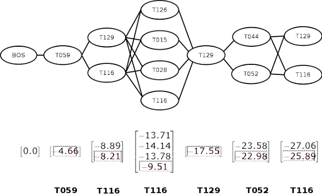
The sequence of entity spans, each mapped to one or more semantic type codes can be represented by a graph of semantic type nodes as shown below. Here, each vertical grouping corresponds to an entity position. The BOS node is a special node representing the beginning of the sequence. Based on our intuition above, entity disambiguation is now just a matter of finding the most likely path through the graph.


Of course, "most likely" implies that we need to know the probabilities for transitioning between semantic types. We can think of the graph as a Markov Chain, and consider the probability of each node in the graph as being determined only by its previous node. Fortunately, this information is already available as a result of the NER + NEL process for the entire CORD-19 dataset, where approximately half of the entity spans mapped unambiguously to a single UMLS concept. Most concepts map to a single semantic type, but in cases where they map to multiple, we consider them as separate records. We compute pairwise transition probabilities across semantic types for these unambiguously linked pairs across the CORD-19 dataset and create our transition matrix. In addition, we also create a matrix of emission probabilities that identify the probabilities of resolving to a concept given a semantic type. 

Using the transition probabilities, we can traverse each path in the graph from starting to ending position, computing the path probability as the product of transition probabilities (or for computational reasons, the sum of log-probabilities) of the edges. However, better methods exist, such as the Viterbi algorithm, which allows us to save on repeated computation of common edge sequences across multiple paths. This is what we used to compute the most likely path through our semantic type graph. 

The Viterbi algorithm consists of two phases -- forward and backward. In the forward phase, we move left to right, computing the log-probability of each transition at each step, as shown by the vectors below each position in the figure. When computing the transition from multiple nodes to a single node (such as the one from [T129, T116] to [T126], we compute for both paths and choose the maximum value. 

In the backward phase, we move from right to left, choosing the maximum probability node at each step. This is shown in the figure as boxed entries. We can then lookup the appropriate semantic type and return the most likely sequence of semantic types (shown in bold in the bottom of the figure). 

However, our objective is to return disambiguated concept linkages for entities. Given a disambiguated semantic type and multiple possibilities indicated by SciSpacy's linking process, we use the emission probabilities to choose the most likely concept to apply at the position. The result for our example is shown in the table below.

Entity-ID Entity Span Concept-ID Concept Primary Name Semantic Type Code Semantic Type Name Correct?
1 staining C0487602 Staining method T059 Laboratory Procedure N/A*
2 antibodies C0003241 Antibodies T116 Amino Acid, Peptide, or Protein Yes
3 cat C0008169 Chloramphenicol O-Acetyltransferase T116 Amino Acid, Peptide, or Protein No
4 antigens C0003320 Antigens T129 Immunologic Factor N/A*
5 binding C1145667 Binding action T052 Activity Yes
6 antibodies C0003241 Antibodies T116 Amino Acid, Peptide, or Protein Yes
(N/A: non-ambiguous mappings) 

I thought this might be an interesting technique to share, hence writing about it. In addition, in the spirit of reproducibility, I have also provided the following artifacts for your convenience.
  1. Code: This github gist contains code that illustrates NER + NEL on an input sentence using SciSpacy and its UMLS integration, and then applies my adaptation of the Viterbi method (as described in this post) to disambiguate ambiguous entity linkages.
  2. Data: I have also provided the transition and emission matrices, and their associated lookup tables, for convenience, as these can be time consuming to generate from scratch from the CORD-19 dataset.
As always, I appreciate your feedback. Please let me know if you find flaws with my approach, and/or you know of a better approach for entity disambiguation

Monday, December 09, 2019

PyData LA 2019: Trip Report


PyData LA 2019 was last week, and I had the opportunity to attend. I also presented about NERDS (Named Entity Recognition for Data Scientists), an open source toolkit built by some colleagues from our Amsterdam office. This is my trip report.

The conference was three days long, Tuesday to Thursday, and was spread across 3 parallel tracks. So my report is necessarily incomplete, and limited to the talks and tutorials I attended. The first day was tutorials, and the next two days were talks. In quite a few situations, it was tough to choose between simultaneous talks. Fortunately, however, the talks were videotaped, and the organizers have promised to put them up in the next couple of weeks, so looking forward to catching up on the presentations I missed. The full schedule is here. I am guessing attendees will be notified by email when videos are released, and I will also update this post when that happens.

Day 1: Tutorials


For the tutorials, I did all the tutorials in the first track. Of these, I came in a bit late for Computer Vision with Pytorch, since I miscalculated the volume (and delaying power) of LA Traffic. It was fairly comprehensive, although I was familiar with at least some of the material already, so in retrospect, I should probably have attended one of the other tutorials.

The second tutorial was about Kedro and MLFlow and how to combine the two to build reproducible and versioned data pipelines. I didn't know that MLFlow can be used standalone outside Spark, so definitely something to follow up there. Kedro looks like scaffolding software which allows users to hook into specific callback points in its lifecycle.

The third tutorial was a presentation on teaching a computer to play PacMan using Reinforcement Learning (RL). RL apps definitely have a wow factor, and I suppose it can be useful where the environment is deterministic enough (rules of a game, laws of physics, etc.), but I often wonder if we can use it to train agents that can operate in a more uncertain "business applications"-like environment. I am not an expert on RL though, so if you have ideas on how to use RL in these areas, I would appreciate learning about them.

The fourth and last tutorial of the day was Predicting Transcription Factor (TF) genes from genetic networks using Neural Networks. The data extraction process was pretty cool, it was predicated on the fact that TF genes typically occupy central positions in genetic networks, so graph based algorithms such as connectedness and Louvain modularity can be used to detect them in these networks. These form the positive samples, and standard negative sampling is done to extract negative samples. The positive records (TFs) are oversampled using SMOTE. Features for these genes come from an external dataset of 120 or so experiments, where each gene was subjected to these experiments and results recorded. I thought that the coolest part was using the graph techniques for building up the dataset.

Days 2 and 3: Talks


All the talks provided me with some new information in one form or the other. In some cases, it was a tough choice to make, since multiple simultaneous talks seemed equally interesting to me going in. Below I list the ones I attended and liked, in chronological order of appearance in the schedule.

  • Gradient Boosting for data with both numerical and text features -- the talk was about the CatBoost library from Yandex, and the talk focused on how much better CatBoost is in terms of performance (especially on GPU) compared to other open source Gradient Boosting libraries (LightGBM and one other that I can't recall at the moment). CatBoost definitely looks attractive, and at some point I hope to give it a try.
  • Topological Techniques for Unsupervised Learning -- talked about how the topological technique called Uniform Manifold Approximation and Projection (UMAP) for dimensionality reduction can be used for generating very powerful embeddings and for clustering that is competitive with T-SNE. UMAP is more fully described in this paper on arXiv (the presenter was one of the co-authors of this paper). There was one other presentation on UMAP by one of the other co-authors which I was unable to attend.
  • Guide to Modern Hyperparameter Tuning Algorithms -- presented the open source Tune Hyperparameter Tuning Library from the Ray team. As with the previous presentation, there is a paper on arXiv that describes this library in more detail. The library provides functionality to do grid, random, bayesian, and genetic search over the hyperparameter space. It seems to be quite powerful and easy to use, and I hope to try it out soon.
  • Dynamic Programming for Hidden Markov Models (HMM) -- one of the clearest descriptions of the implementation of the Viterbi (given the parameters for the model and the observed states, find the most likely sequence of hidden states) algorithm that I have ever seen. The objective is for the audience to understand HMM (specifically Viterbi algorithm) well enough so they can apply it to new domains where it might be applicable.
  • RAPIDS: Open Source GPU Data Science -- I first learned about NVidia's RAPIDS library at KDD 2019 earlier this year. RAPIDS provides GPU optimized drop-in replacements for NumPy, Pandas, Scikit-Learn, and NetworkX (cuPy, cuDF, cuML, and cuGraph), which run order of magnitude faster if you have a GPU. Unfortunately, I don't have a GPU on my laptop, but the presenter said that images with RAPIDS pre-installed are available on Google Cloud (GCP), Azure, and AWS.
  • Datasets and ML Model Versioning using Open Source Tools -- this is a presentation on the Data Version Control (DVC) toolkit, which gives you a set of git like commands to version control your metadata, and link them to a physical file on some storage area like S3. We had envisioned using it internally for putting our datasets and ML models under version control some time back, so I was familiar with some of the information provided. But I thought the bit about creating versioned ML pipelines (data + model(s)) was quite interesting.

And here are the talks I would like to watch once the videos are uploaded.

  • Serverless Demo on AWS, GCP, and Azure -- this was covered in the lightning round on the second day. I think this is worth learning, since it seems to be an easy way to set up demos that work on demand. Also learned about AWS Batch, a "serverless" way to serve batch jobs (or at least non-singleton requests).
  • Supremely Light Introduction to Quantum Computing -- because Quantum Computing which I know nothing about.
  • Introducting AutoImpute: Python package for grappling with missing data -- No explanation needed, clearly, since real life data often comes with holes, and having something like this gives us access to a bunch of "standard" strategies fairly painlessly.
  • Tackling Homelessness with Open Data -- I would have attended this if I had not been presenting myself. Using Open Data for social good strikes me as something we, as software people, can do to improve our world and make it a better place, so always interested in seeing (and cheering on) others who do it.
  • What you got is What you got -- speaker is James Powell, a regular speaker I have heard at previous PyData conferences, who always manages to convey deep Python concepts in a most entertaining way.
  • GPU Python Libraries -- this was presented by another member of the RAPIDS team, and according to the previous presenter, focuses more on the Deep Learning aspect of RAPIDS.

And then of course there was my presentation. As I mentioned earlier, I spoke of NERDS, or more specifically my fork of NERDS where I made some improvements on the basic software. The improvements started as bug fixes, but currently there are quite a few significant changes, and I plan on making a few more. The slides for my talk are here. I cover why you might want to do Named Entity Recognition (NER), briefly describe various NER model types such as gazetteers, Conditional Random Fields (CRF), and various Neural model variations around the basic Bidirectional LSTM + CRF, cover the NER models available in NERDS, and finally describe how I used them to detect entities in a Biological Entity dataset from BioNLP 2004.

The reason I chose to talk about NERDS was twofold. First, I had begun to get interested in NERs in general in my own work, and "found" NERDS (although since it was an OSS project from my own company, not much discovery was involved :-)). I liked that NERDS does not provide "new" ML models, but rather a unified way to run many out of the box NER models against your data with minimum effort. In some ways, it is a software engineering solution that addresses a data science problem, and I thought the two disciplines coming together to solve a problem was an interesting thing in itself to talk about. Second, I feel that custom NER building is generally considered something of a black art, and something like NERDS has the potential to democratize the process.

Overall, based on some of the feedback I got on LinkedIn and in person, I thought the presentation was quite well received. There was some critical feedback saying that I should have focused more on the intuition behind the various NER modeling techniques than I did. While I agree that this might be desirable, I had limited time to deliver the talk, and I would not have been able to cover as much if I spent too much time on basics. Also, since the audience level was marked as Intermediate, I risked boring at least part of the audience if I did so. But I will keep this in mind for the future.

Finally, I would be remiss if I didn't mention all the wonderful people I met at this conference. I will not call you out by name, but you know who you are. Some people think of conferences as places where a small group of people get to showcase their work in front of a larger group of people, it is also a place where you get to meet people in your discipline but in similar or different domains, and I find it immensely helpful and interesting to share ideas and approaches for solving different problems.

And that's all I have for today. I hope you enjoyed reading my trip report.


Friday, August 09, 2019

KDD 2019: Trip Report


I had the good fortune last week to attend KDD 2019, or more formally, the 25th ACM SIGKDD Conference on Knowledge Discovery and Data Mining, that was held at downtown Anchorage, AK from August 4-8, 2019. Approximately 3000 participants descended on the city (boosting the population by 1%, as Mayor Berkowitz pointed out in his keynote). This was my first KDD, and I found it somewhat different from other conferences I have attended in the past. First, there seems to be a more equitable representation from academia and industry. To some extent this is understandable, since data is a big part of KDD, and typically, it is industry that collects, and has access to, large and interesting datasets. A side effect is that there is as much emphasis on tools and frameworks as on methods, so by judiciously selecting the sessions you attend, you could load up on the combination that works best for you. Second, there is a surfeit of choice -- at any point in time during the conference, there were 5-8 parallel tracks spread across two conference buildings. While there were some difficult choices to make as to which track to attend and which to drop, I felt I got a lot of value out of the conference. Of course, this does mean that each attendee's experience of the conference is likely to be somewhat personalized by their background and their choices. In this post, I will write about my experience at KDD 2019.

Day 1 (Sunday, August 4) -- Lecture Style Tutorials


My choices here were slightly non-obvious, since I haven't worked directly with hospital data (unless you count the i2b2 and MIMIC datasets), and don't forsee doing so any time soon. However, I had just finished reading the book Deep Medicine by Dr. Eric Topol, and was quite excited about all the cool ideas in the book around using machine learning to assist medical practitioners in hospital settings. There were tutorials that were closer to my work interests, but I figured that it might be good to mix in some exploration with the exploitation, and I decided to attend the tutorials on Mining and model understanding on medical data, and Data mining methods for Drug Discovery and Development.

The first tutorial provided a very broad coverage of Medical Data Mining, starting with sources and coding schemes (ICD-10, ATC, etc.), various interesting strategies for extracting temporal features from Electronic Health Records (EHR), such as the use of Allen's temporal logic and Itemset disproportionality. Also covered were Learning from Cohorts and the use of Randomized Control Trials, and the application of the Dawid-Skene algorithm to Data Fusion, i.e., a process of creating clean features from multiple noisy features, which reminded me of the Snorkel generative model. I also learned that the Dawid-Skene algorithm is equivalent to a one-layer Restricted Boltzmann Machine (RBM) (example code in Tensorflow). Another interesting insight provided by one of the presenters is the timeline for ML techniques -- starting with rules, then simple matrix based techniques (logistic regression, decision trees, SVM, XGBoost, etc), then very briefly probabilistic statistical techniques, rapidly supplanted by Deep Learning techniques. There is of course a move to merge the last two techniques nowadays, so probabilistic techniques are coming back to the forefront. The tutorial was run by Prof. Myra Spiliopoulou and her team from the Otto-von-Guericke-Universität Magdeburg.

The second tutorial provided a broad overview of in-silico drug development. Primary tasks here are Molecular Representation Learning (for example, mol2vec) to allow molecules to be represented in a semantic vector space similar to word embeddings; Molecular Property Prediction that takes a drug molecule and outputs its property; Drug Repositioning that takes a (molecule, protein) pair and outputs an affinity score to indicate how the molecule will interact with the (disease) protein; Adverse Drug Interation that takes a (molecule, molecule) pair and predicts their interaction; and finally De Novo drug development, which takes a chemical property and outputs a drug molecule. We also learned various schemes for encoding molecules as text, such as 1D, 2D, and 3D encoding, circular fingerprints (ECFPx), SMILES, and adjacency matrix (Bond Adjacency). The main takeaways for me were the ways in which molecules can be encoded and embedded, and the use of Variational Autoencoders (VAE) and grammar constraints to restrict generated drugs to valid ones. The tutorial was run by Cao Xiao and Prof. Jimeng Sun of IQVIA and Georgia Tech respectively.

Day 2 (Monday, August 5) -- Workshops


The workshop I attended was Mining and Learning with Graphs Workshop (MLG 2019). This was an all-day event, with 5 keynote speakers. The first keynote speaker was Prof. Lisa Getoor of University of California, Santa Cruz - she gave a shorter version of her RecSys 2018 keynote and mentioned the Probabilistic Soft Logic (PSL) Framework, a framework for developing (specifying rules and optimizing) probabilistic models. Prof. Austin Benson from Cornell spoke of Higher Order Link Prediction (slides). Lada Adamic spoke about interesting Social Network findings based on crunching county-level US demographics data from Facebook. She works for Facebook now, but I remember her as the University of Michigan professor who re-introduced me to Graph Theory after college, through her (now no longer active) course on Social Network Analysis on Coursera. Prof. Vagelis Papalexakis, from the University of Riverside, talked about Tensor Decomposition for Multi-aspect Graph Analytics, a talk that even a fellow workshop attendee and PhD student who had a poster accepted thought was heavy. Finally, Prof Huan Liu of Arizona State University, and the author of the (free to download) book Social Media Mining, spoke very entertainingly about the challenges in mining Big Social Media data, mostly related to feature sparsity and privacy, and possible solutions to these. He also pointed the audience to an open source feature selection library called scikit-feature.

There were quite a few papers in there (as well as posters) in the workshop that I found interesting. The paper Graph-Based Recommendation with Personalized Diffusions uses random walks to generate personalized diffusion features for an item-based recommender. The Sparse + Low Rank trick for Matrix Factorization-based Graph Algorithms based on Halko's randomized algoithm, describes a simple way to make matrix factorization more scalable by decomposing the matrix into a sparse and a low-rank component. Graph Embeddings at Scale proposes a distributed infrastructure to build graph embeddings that avoids graph partitioning. The Temporal Link Prediction in Dynamic Networks (poster) uses a SiameseLSTM network to compare pairs of sequences of node embeddings over time. When to Remember where you came from: Node Representation Learning in Higher-Order Networks uses historical links to predict future links.

Finally, I also went round looking at posters from other workshops. Of these, I found Automatic Construction and Natural-Language Description of Nonparametric Regression Models that attempts to classify time series trends against a library of reference patterns, and then create a vector that can be used to generate a set of explanations for the trend.

This was followed by the KDD opening session, where after various speeches by committee members and invited dignitaries, awards for various activities were given out. Of note was the ACM SIGKDD Innovation Award awarded to Charu Aggarwal, the ACM SIGKDD Service Award for Balaji Krishnapuram, and the SIGKDD Test of Time Award to Christos Faloutsos, Natalie Glance, Carlos Guestrin, Andreas Krause, Jure Leskovec, and Jeanne VanBriesen.

There was another poster session that evening, where I had the chance to see quite a few more posters. Some of these that I found interesting are as follows. Revisiting kd-tree for Nearest Neighbor Search, which uses randomized partition trees and Fast Fourier Transforms (FFT) to more efficiently build kd-trees with the same level of query accuracy. It caught my interest because I saw something about randomized partition trees, and I ended up learning something interesting. Another one was Riker: Mining Rich Keyword Representations for Interpretable Product Question answering, which involves creating word vectors for questions and using attention maps to predict the importance of each of these words for a given product.

Day 3 (Tuesday, August 6) -- Oral Presentations


The day started with a keynote presentation titled The Unreasonable Effectiveness and Difficulty of Data in Healthcare by Dr Peter Lee of Microsoft Research. To a large extent, his points mirror those made by Dr. Eric Topol in Deep Medicine in terms of what is possible in medicine with the help of ML/AI, but he also looks at the challenges that must be overcome before this vision becomes reality.

Following that, I attended two sessions of Applied Data Science Oral Presentations, one on Auto-ML and Development Frameworks, and the other on Language Models and Text Mining, and then one session of Research Track Oral Presentation on Neural Networks.

I found the following papers interesting in the first Applied Data Science session. Auto-Keras: An Efficient Neural Architecture Search System uses Bayesian Optimization to find the most efficient Dense Keras network for your application. To the user, calling this is a one-liner. Currently this works on legacy Keras, but the authors are working with Google to have this ported to tf.keras as well. A more interesting framework keras-tuner currently works with tf.keras, and while invoking keras-tuner involves more lines of code, it does seem to be more flexible as well. TF-Ranking: Scalable Tensorflow Library for Learning-to-Rank is another Learning to Rank (LTR) framework that is meant to be used instead of libraries like RankLib or LambdaMART. It provides pointwise, pairwise based, and listwise ranking functions. FDML: A Collaborative Machine Learning Framework for Distributed Learning is meant to be used where learning needs to happen across platforms which are unable to share data either because of volume or privacy reasons. The idea is to learn local models with diverse local features, which will output local results, then combine local results to get the final prediction. In addition, there was a talk on Pythia: AI assisted code completion system that is used in the VSCode editor, and Shrinkage Estimators in Online Experiments, which mentions the Pytorch based Adaptive Experimentation Platform for Bayesian Parameter Optimization.

The second Applied Data Science session was on Language Models. The papers I found interesting in this session are as follows. Unsupervised Clinical Language Translation (paper) which uses an unsupervised technique to induce a dictionary between clinical phrases and corresponding layman phrases, then uses a standard Machine Translation (MT) pipeline to translate one to the other. A reverse pipeline is also constructed, which can be used to generate more training data for the MT pipeline. GMail Smart Compose: Real-Time Assisted Writing underlies the phrase completion feature most GMail users are familiar with. It is achieved by interpolating predictions from a large global language model and a smaller per-user language model. As part of this work, they have open sourced Lingvo, a Tensorflow based framework for building sequence models. And finally, Naranjo Question Answering using End-to-End Multi-task Learning Model attempts to infer adverse drug reactions (ADR) from EHRs by answering the Naranho questionnaire using automated question answering. There was also Automatic Dialog Summary Generation for Customer Service uses key point sequences to guide the summarization process, and uses a novel Leader-Writer network for the purpose.

The final oral presentation session for the day was the Research Track on Neural Networks. Unfortunately, I did not find any of the papers useful, in terms of techniques I could borrow for my own work. I did get the impression that Graph based Neural Networks were the new thing, since almost every paper used some form of Graph network. Apart from graph embeddings that are derived from node properties or conducting random walks on graphs, there is the graph convolution network (GCN) which uses graph local features instead of spatially local features. The GCN-MF: Disease-Gene Association Identification by Graph Convolutional Networks and Matrix Factorization uses this kind of architecture to detect associations between diseases and genes. Similarly, the Origin-destination Matrix prediction via Graph Convolution: A new perspective of Passenger Demand Modeling uses GCNs to predict demand for ride-hailing services.

The exhibition booth had also opened earlier that day, so I spent some time wandering the stalls, meeting a few people and asking questions about their products. There were a couple of publishers, MIT Press and Springer, selling Data Science books. There were some graph database companies, TigerGraph and Neo4j. Microsoft and Amazon were the two cloud providers with booths, but Google wasn't present (not my observation, it was pointed out to me by someone else). Indeed and LinkedIn were also there. NVIDIA was promoting its RAPIDS GPU-based acceleration framework, along with its GPUs. There were a bunch of smaller data science / analytics companies as well. I picked up a couple of stickers and some literature from the National Security Agency (NSA) and the NVIDIA booths.

I then wandered over to the poster area. I managed to talk to a few people and listen to a few presentations. Notable among them was the poster on Chainer: a Deep Learning Framework for Accelerating the Research Cycle. I haven't used Chainer, but looking at the code in the poster, it looked a bit like Pytorch (or more correctly perhaps, Pytorch looks a bit like Chainer). Another framework to pick up when time permits, hopefully.

Day 4 (Wednesday, August 7) -- Hands-on Tutorials


I came in bright and early, hoping to attend the day's keynote presentation, but ended up having a great conversation with a data scientist from Minnesota instead, as we watched the sun rise across the Alaska range from the third floor terrace of the conference building. In any case, the keynote I planned on attending ended up getting cancelled, so it was all good. For my activity that day, I had decided on attending two hands-on tutorials, one about Deep Learning for Natural Language Processing with Tensorflow, and the other about Deep Learning at Scale on Databricks.

The Deep Learning for NLP with Tensorflow was taught by a team from Google. It uses the Tensorflow 2.x style of eager execution and tf.keras. It covers basics, then rapidly moves on to sequence models (RNN, LSTM), embeddings, sequence to sequence models, attention, and transformers. As far as teachability goes, I have spent a fair bit of time trying to figure this stuff out myself, then trying to express it in the cleanest possible way to others, and I thought this was the most intuitive explanation of attention I have seen so far. The slide deck is here, they contain links to various Collab notebooks. The Collab notebooks can also be found at this github link. The tutorial then covers the transformer architecture, and students (in an ideal world with enough internet bandwidth and time) are taught how to construct a transformer encoder-decoder architecture from scratch. They also teach you how to user the pre-trained BERT model from TF-Hub and optionally fine tune it. Because we were not in an ideal world, after the initial few Collab notebooks, it was basically a lecture, where we are encouraged to run the notebooks on our own time.

The Deep Learning at Scale on Databricks was taught by a team from Databricks, and was apparently Part-II in a two part session. But quite a few of us showed up based on the session being marked as a COPY of the morning session, so the instructor was kind enough to run through the material again for our benefit. The slide deck can be found here. Unfortunately, I can no longer locate the URL for the notebook file archive to be imported into Databricks, but I am guessing these notebooks will soon be available as a Databricks tutorial. We used the Databricks platform provided by Microsoft Azure. In any case, the class schedule was supposed to cover Keras basics, MLFlow, Horovod for distributed model training, HyperOpt for simultaneously training models on workers with different hyperparameters. We ended up running through the Keras basics very fast, then spending some time on MLFlow, and finally run distributed training with Horovod on Spark. Most people had come to get some hands-on with Horovod anyway, so not being able to cover HyperOpt was not a big deal for most of us.

That evening was also the KDD dinner. I guess lot of people (including me, based on past ACL conferences) had expected something more formal, but it turned out to be a standup with drinks and hors-d'oeuvres. To be fair, the stand-up model does give you more opportunities to network. However, it was also quite crowded, so after a fairly long time spent in lines with correspondingly little profit, I decided to hit the nearby Gumbo House where I enjoyed a bowl of gumbo and some excellent conversation with a couple of AWS engineers, also KDD attendees who decided to eat out rather than braving the lines. Talking of food, other good places to eat at Anchorage downtown are the Orso, Pangea, and Fletcher's (good pizza). I am sure there are others, but these are the ones I went to and can recommend.

Day 5 (Thursday, August 8) -- More Hands-on Tutorial


This was the last day of the conference. I had a slightly early flight (3 pm) which meant that I would be able to attend only sessions in the first half. In the morning keynote, Prof. Cynthia Rudin of Duke University spoke about her experience with smaller simpler models versus large complex ones, and made the point that it is harder to come up with a simple model because the additional constraints are harder to satisfy. She then shows that it is possible to empirically test for whether one or more simple models are available by looking at accuracies from multiple ML models. Overall, a very thought provoking and useful talk.

For the rest of the day, I chose another hands-on tutorial titled From Graph to Knowledge Graph: Mining Large-scale Heterogeneous Networks using Spark taught by a team from Microsoft. As with the previous hands-on, we used Databricks provided by Azure. The objective was to learn to operate on subsets of the Microsoft Academic Graph, using Databricks notebooks available on this github site. However, since we were all sharing a cluster, there wasn't enough capacity for the students to do any hands-on, so we ended up watching the instructor run through the notebooks on the projector. The initial notebooks (run before lunch) seemed fairly basic, with standard DataFrame operators being used. I am guessing the fun stuff happened in the afternoon after I left, but in any case, Microsoft also offers a longer course From Graph to Knowledge Graph - Algorithms and Applications on edX, which I plan on auditing.

Closing Thoughts


There were some logistical issues, that in hindsight perhaps, could be avoided. While Anchorage is a beautiful city and I thoroughly enjoyed my time there, for some attendees it was perhaps not as great an experience. One particularly scary problem was that some people's hotel bookings got cancelled due to a mixup with their online travel agents, which meant that they had no place to sleep when they arrived here. Apparently some people had to sleep on park benches -- I thought that was particularly scary, at least until the University of Alaska opened up their dormitory to accommodate the attendees who had nowhere to go. I didn't get accommodation at the "KDD approved" hotels listed on their site either, but I did end up getting a place to stay that was only a 7 minute walk from the conference venue, so I count myself as one of the lucky ones. However, apart from this one major mishap, I think the conference went mostly smoothly.

At RecSys 2018, which I attended last year, one of the people in the group I found myself in said that he had finally "found his people". While my conference experience has been improving steadily over time with respect to the social aspect, and I did end up making lot more friends at RecSys 2018 than I did here (partly due to the network effect of my colleague and his friends being die-hard extroverts), I do think I have finally found mine at KDD.


Saturday, August 11, 2018

Keyword deduplication using the Python dedupe library


I have been experimenting with keyword extraction techniques against the NIPS Papers dataset, consisting of titles, abstracts and full text of all papers from the Neural Information Processing Systems (NIPS) conference from 1987-2017, and contributed by Ben Hamner. The collection has 7239 papers written by 9785 authors. The reason I preferred this dataset to others such as Reuters or Medline is because it is smaller, and I can be both programmer and domain expert, and because I might learn interesting things while combing through the text of the papers looking for patterns to exploit.

In order to generate keywords, I used Ted Dunning's Log Likelihood Ratio (LLR) method (blog post, paper (PDF)) and the RAKE algorithm (described in Pattern Recognition and Machine Learning by Christopher Bishop, and adapted from code at aneesha/RAKE). I then selected the top scoring keywords from both methods, merged them to remove duplicate suggestions, went through them manually to remove what I considered spurious keywords (things like "et al", "better proposals", "usually set conservatively", etc), and then trained a MAUI model (following this blog post by Alyona Medelyan, creator of MAUI) using these keywords and the text. I then turned around and used the model to predict keywords against the same text (hoping to extract some more keywords that were missed in the training set). I then merged the predicted keywords with the training keywords.

The next step was to remove obviously duplicate keywords, such as singular and plural versions of the same thing ("absolute value", "absolute values"), words that were spelled differently but meant the same ("datasets", "data sets"), words that were close enough in meaning to appear as duplicates ("local linear", "locally linear"), etc. At this point, I had only about 2281 keywords, so I could have just done brute force matching (i.e., run 2281x2281 comparisons across all keywords), but I had recently heard about the Python Dedupe Library from Anne Moshyedi and Taylor Kramer, University of Virginia (UVA) Computer Science students interning at SWIFT Innovation Labs, who I was collaborating with around my open source project Solr Dictionary Annotator (SoDA) and wanted to try it out. They were using it as a step in their pipeline to resolve entities in structured data, which looks like the suggested use case for dedupe, going by the examples at their examples repository dedupeio/dedupe-examples. This post is about using dedupe against this set of keywords.

Since keywords are just text data, the first step was to convert it to some kind of structured data. For that I chose to generate 3-character shingles from the data, then run it through a feature hasher to hash these shingles down to a fixed length vector. Here is the code to do that.

1
 2
 3
 4
 5
 6
 7
 8
 9
10
11
12
13
14
15
16
17
18
import nltk
import numpy as np
import os

from sklearn.feature_extraction import FeatureHasher
from sklearn.metrics import jaccard_similarity_score

hasher = FeatureHasher(input_type="string", n_features=25, dtype=np.int32)
keywords = ["absolute value", "absolute values"]
hashes = []
for keyword in keywords:
    shingles = ["".join(trigram) for trigram 
        in nltk.trigrams([c for c in keyword])]
    keyword_hash = hasher.transform([shingles]).toarray()
    hashes.append(keyword_hash)
    print(keyword, keyword_hash)

print("jaccard:", jaccard_similarity_score(hashes[0][0], hashes[1][0]))

The output shows that we don't lose too much information after the feature hashing, the Jaccard similarity between the two fixed length (size 25) hashes for the two strings "absolute value" and "absolute values" is 0.96.

1
2
3
absolute value : [0, 0, 1, 0, 0, 0, 0, -1, -1, 0, 0, -1, 0, 0, 0, 0, 0, 0, 0, -2, -1, 0, 1, 0, 0]
absolute values: [0, 0, 1, 0, 0, 0, 0, -2, -1, 0, 0, -1, 0, 0, 0, 0, 0, 0, 0, -2, -1, 0, 1, 0, 0]
jaccard similarity: 0.96

We then apply this feature hashing procedure to all our keywords and write these hashes out to a CSV file along with the original keyword. Originally I added the keyword because there is an active learning component in the dedupe pipeline where the user is asked to identify if a pair of records are duplicates or not, and having the original keyword show up is the easiest way for the human trainer to identify duplicates. Later I realized that the keyword string is a useful feature by itself, because dedupe contains functionality to match against strings inside structured input as well.

1
 2
 3
 4
 5
 6
 7
 8
 9
10
11
12
13
14
15
16
17
18
19
20
21
22
23
24
25
26
27
28
29
DATA_DIR = "../data"

CURATED_KEYWORDS = os.path.join(DATA_DIR, "raw_keywords.txt")
CURATED_KEYWORD_HASHES = os.path.join(DATA_DIR, "curated_keywords_hash.csv")

fcurated = open(CURATED_KEYWORDS, "r")
fhashed = open(CURATED_KEYWORD_HASHES, "w")

# header
cols = ["id"]
cols.extend(["col_{:d}".format(i+1) for i in range(25)])
cols.append("keyword")
fhashed.write("{:s}\n".format(",".join(cols)))

# shingle each word into 3-char trigrams, then hash to 25 features
hasher = FeatureHasher(input_type="string", n_features=25, dtype=np.int32)
for rowid, keyword in enumerate(fcurated):
    keyword = keyword.strip()
    shingles = ["".join(trigram) for trigram 
        in nltk.trigrams([c for c in keyword])]
    keyword_hash = hasher.transform([shingles]).todense().tolist()[0]
    cols = [str(rowid)]
    cols.append(",".join([str(h) for h in keyword_hash]))
    cols.append(keyword)
    fhashed.write("{:s}\n".format(",".join(cols)))

fhashed.close()
fcurated.close()
print("num keywords: {:d}".format(rowid))

Next we take this set of deduped 2281 keywords, and run it through the dedupe pipeline. The code below is adapted from and mimics closely the CSV example on the dedupe-examples site. Dedupe is a machine learning pipeline that uses a combination of blocking (or grouping by fields), hierarchical clustering and logistic regression, along with active learning, to come up with its results.

The first step in the training is for the user to tell dedupe what fields to pay attention to during the deduping process. In our case, it is every element of the feature hasher output (represented by col_1 through col_25) plus the keyword string. Using this information, dedupe will identify potential duplicate pair candidates and ask the user for confirmation, a process it calls active labeling. During this phase, dedupe writes out a settings file (dedupe_keywords_learned_settings) and label file (dedupe_keywords_training.json). The code below checks for the presence of these files, and if found, it will skip the active labeling step (so for retraining, you should remove these files).

Once the active labeling, blocking and clustering is done, the predicted duplicate pairs can be retrieved from the dedupe classifier by supplying a threshold, essentially telling it how much more you value recall over precision. The last block of code below just retrieves these candidate pairs and outputs it into a tab separated format into the file keyword_dedup_mappings.tsv. I sort the keywords so that the longer one is first in the pair, that is to accomodate the next step in this pipeline which I will not go into in this post.

1
 2
 3
 4
 5
 6
 7
 8
 9
10
11
12
13
14
15
16
17
18
19
20
21
22
23
24
25
26
27
28
29
30
31
32
33
34
35
36
37
38
39
40
41
42
43
44
45
46
47
48
49
50
51
52
53
54
55
56
57
58
59
60
61
62
63
64
65
66
67
68
69
70
71
import csv
import os
import dedupe

DATA_DIR = "../data"
MODEL_DIR = "../models"

RAW_INPUT = os.path.join(DATA_DIR, "curated_keywords_hash.csv")
SETTINGS_FILE = os.path.join(MODEL_DIR, "dedupe_keywords_learned_settings")
TRAINING_FILE = os.path.join(MODEL_DIR, "dedupe_keywords_training.json")
OUTPUT_FILE = os.path.join(DATA_DIR, "keyword_dedupe_mappings.tsv")

# read training file (written using 09-keyword-dedupe) and transform
# into format suitable for use by dedupe
data = {}
with open(RAW_INPUT, "rb") as csvfile:
    reader = csv.DictReader(csvfile)
    for row in reader:
        row_id = int(row["id"])
        data[row_id] = dict(row.items())
        
# training
if os.path.exists(SETTINGS_FILE):
    print("reading from settings file {:s}".format(SETTINGS_FILE))
    with open(SETTINGS_FILE, "rb") as f:
        deduper = dedupe.StaticDedupe(f)
else:
    # define fields for deduper to pay attention to, here we
    # will ask for all fields except id
    field_names = ["col_{:d}".format(i+1) for i in range(25)]
    fields = [{"field": field_name, "type": "Exact"} 
              for field_name in field_names]
    fields.append({"field": "keyword", "type": "String"})
    deduper = dedupe.Dedupe(fields)
    # feed the deduper a sample of records for training
    deduper.sample(data, 15000)
    # use training data for previous run if available
    if os.path.exists(TRAINING_FILE):
        print("reading labeled examples from training file: {:s}"
              .format(TRAINING_FILE))
        with open(TRAINING_FILE, "rb") as f:
            deduper.readTraining(f)

    # active learning
    print("starting active labeling...")
    dedupe.consoleLabel(deduper)

    deduper.train()            
    
    # save training data to disk
    with open(TRAINING_FILE, "w") as f:
        deduper.writeTraining(f)
    with open(SETTINGS_FILE, "w") as f:
        deduper.writeSettings(f)
        
# blocking
print("blocking...")
threshold = deduper.threshold(data, recall_weight=1.5)

# clustering
print("clustering...")
clustered_dupes = deduper.match(data, threshold)

# write results
with open(OUTPUT_FILE, "w") as f:
    for cluster_id, cluster in enumerate(clustered_dupes):
        id_set, scores = cluster
        keywords = sorted([data[id]["keyword"] for id in id_set],
                          key=lambda x: len(x), reverse=True)
        f.write("{:s}\t{:s}\t{:.3f}\n".format(
            keywords[0], keywords[1], scores[0]))

The active learning part shows a pair of records on the console and asks the user to say yes or no to whether these records should be considered the same. User can exit the training loop at any point by choosing finish, or ignore a record as well by choosing unsure. This is done by the consoleLabel convenience method. The recommendation is to train 10 records, but I ended up training close to 40 because I wanted to give it an even split of positive and negative examples. Here is what a single query looks like.

1
 2
 3
 4
 5
 6
 7
 8
 9
10
11
12
13
14
15
16
17
18
19
20
21
22
23
24
25
26
27
28
29
30
31
32
33
34
35
36
37
38
39
40
41
42
43
44
45
46
47
48
49
50
51
52
53
54
55
56
57
col_1 : 0
col_2 : 1
col_3 : 0
col_4 : 0
col_5 : 1
col_6 : 0
col_7 : -1
col_8 : 1
col_9 : 0
col_10 : 1
col_11 : 0
col_12 : 0
col_13 : 0
col_14 : 0
col_15 : 0
col_16 : 0
col_17 : 0
col_18 : 0
col_19 : 1
col_20 : -1
col_21 : 0
col_22 : 0
col_23 : 1
col_24 : 2
col_25 : 0
keyword : learning model

col_1 : 0
col_2 : 1
col_3 : 0
col_4 : 0
col_5 : 1
col_6 : 0
col_7 : -1
col_8 : 1
col_9 : 0
col_10 : 1
col_11 : 0
col_12 : 0
col_13 : 0
col_14 : 0
col_15 : 1
col_16 : 0
col_17 : 0
col_18 : 0
col_19 : 1
col_20 : -1
col_21 : 0
col_22 : 0
col_23 : 1
col_24 : 2
col_25 : 0
keyword : learning models

11/10 positive, 19/10 negative
Do these records refer to the same thing?
(y)es / (n)o / (u)nsure / (f)inished / (p)revious

Our final step is evaluating the quality of the predictions that dedupe gave us. Since I am looking for words which are almost duplicates but not quite, the edit distance would be a good way to measure such a thing. Since dedupe reports the confidence score when predicting duplicates, we will consider any pair as a duplicate when predicted with a confidence of over 0.75. Conversely, we will consider a pair real duplicates if the edit distance is upto 2 characters. We have codified this and use the metrics provided by Scikit-Learn to generate evaluation scores.

1
 2
 3
 4
 5
 6
 7
 8
 9
10
11
12
13
14
15
16
17
18
19
20
21
22
23
24
25
26
27
28
29
from sklearn.metrics import accuracy_score, confusion_matrix, classification_report

i = 0
labels, preds = [], []
f = open(KEYWORD_DEDUPE_MAPPINGS, "r")
for line in f:
    keyword_left, keyword_right, score = line.strip().split("\t")
    score = float(score)
    preds.append(1 if score > 0.75 else 0)
    edit_dist = nltk.edit_distance(keyword_left, keyword_right)
    labels.append(1 if edit_dist <= 2 else 0)
    if i <= 10:
        print("{:25s}\t{:25s}\t{:.3f}\t{:.3f}".format(keyword_left, keyword_right, 
                                                      score, edit_dist))
    i += 1
f.close()

acc = accuracy_score(labels, preds)
cm = confusion_matrix(labels, preds)
cr = classification_report(labels, preds)

print("---")
print("accuracy: {:.3f}".format(acc))
print("---")
print("confusion matrix")
print(cm)
print("---")
print("classification report")
print(cr)

The output of this code block is shown below. The first block is the first 10 candidate pairs predicted by dedupe, along with the reported confidence and the computed edit distance. The accuracy of the deduper, given the thresholds, is 0.889 (almost 89%), and the precision, recall and f-score is 0.92, 0.89 and 0.90, all very good, especially given the effort spent in training dedupe.

1
 2
 3
 4
 5
 6
 7
 8
 9
10
11
12
13
14
15
16
17
18
19
20
21
22
23
24
25
26
27
28
learning approaches       learning approach         0.776 2.000
absolute values           absolute value            0.796 1.000
dual variables            dual variable             0.878 1.000
synaptic weights          synaptic weight           0.816 1.000
performance measures      performance measure       0.818 1.000
synthetic dataset         synthetic data            0.684 3.000
dynamical systems         dynamical system          0.836 1.000
action pairs              action pair               0.877 1.000
action potentials         action potential          0.853 1.000
learning models           learning model            0.816 1.000
action spaces             action space              0.816 1.000

---
accuracy: 0.889

---
confusion matrix
[[ 52   5]
 [ 31 235]]

---
classification report
             precision    recall  f1-score   support

          0       0.63      0.91      0.74        57
          1       0.98      0.88      0.93       266

avg / total       0.92      0.89      0.90       323

One small caveat for those of you who are using Anaconda Python 3.x. I am, and I initially tried installing dedupe using pip, but it failed because of some incompatibility with the Anaconda libraries and dedupe-hcluster (a dependency for dedupe). I ended up installing using conda from the derickl repository on my Mac, but that downgraded my Python version from 3 to 2 and broke lots of other code, so I had to reinstall Anaconda (fortunately or unfortunately I have had to do this before and I have the process down, so I was back up and running, including all additional libraries except dedupe, within an afternoon). I ended up installing dedupe on my spare linux box on top of Anaconda Python 2.x using the conda from the riipl-org repository for the linux-64 version of dedupe. I believe that dedupe itself and its dependencies is Python 3 compatible now according to this issue, so hopefully at some point soon dedupe developers will push the latest version to conda-forge for both OSX and Linux.

That's all I have for today. As far as I can see, the dedupe library has been applied to structured data, I haven't seen it applied to unstructured data before, so I hope that the idea of shingling and feature hashing the shingles to convert unstructured to structured tabular data is a useful one for those of you with this use case. I cannot share the code for this at the moment since it is part of a bigger effort that I haven't put on a public repository yet. Once I publish the project, I will update this post with links.


Saturday, March 03, 2018

An implementation of the Silhouette Score metric on Spark


While clustering some data on Spark recently, I needed a quantitative metric to evaluate the quality of the clustering. Couldn't find anything built-in, so (predictably) went looking on Google, where I found this Stack Overflow page discussing this very thing. However, as you can see from the accepted answer, the Silhouette score by definition is not very scalable, since it requires measuring the average distance from each point to every other point in its cluster, as well as the average distance from each point to every other point in all the other clusters. This is clearly an O(N2) operation and not likely to scale for large N. What caught my eye, however, was Geoffrey Anderson's answer, who suggested using the Simplified Silhouette score, which requires only the distance from every point to its own centroid and is thus an O(N) operation and therefore quite scalable.

However, while this is indeed the algorithm suggested in the cited paper (Multiple K Means++ Clustering of Satellite Image Using Hadoop MapReduce and Spark by Sharma, Shokeen and Mathur), this simplified metric only reports on how tight each cluster is. The intent of the original Silhouette score is to report both on tightness of individual clusters as well as separation between clusters. Turns out that such a simplified Silhouette metric does exist, and is defined in detail in this paper titled An Analysis of the Application of Simplified Silhouette to the Evaluation of k-means Clustering Validity (PDF) by Wang, et al. Interestingly, this is also the definition used in the implementation of Silhouette score in Scikit-Learn.

The latter formulation of the Simplified Silhouette Index (SSI) is shown below. For each point i, call the distance to its own cluster centroid ai, and call the distance to the nearest neighboring centroid bi. The Silhouette score for the i-th point is given by SSIi as shown below. Here ai is the indicator of cluster tightness and bi is the indicator of cluster separation. One thing to notice is that in order to compute bi you will need to compute the distance from point i to all the other centroids except its own, so the complexity of the algorithm is O(Nk) where k is the number of clusters — so still linear, but can be high for large k.


Values for SSI can vary in the range [-1, 1]. Values near 0 indicate overlapping clusters, and negative values generally indicate that the point has been wrongly clustered, since it is closer to a different cluster than it's own. Best values of SSI are close to 1. The average SSI across all the points in the corpus gives us an indication of how good the cluster is.

In addition, the distribution of SSI values in each cluster can be histogrammed as shown in this KMeans clustering and Silhouette analysis example on Scikit-Learn. A Clustering where the points are distributd approximately equally across clusters tend to be better, given similar values of average SSI.

A flow diagram for my implementation is shown below. There are 3 inputs needed, an RDD of point vectors keyed by an sequential record ID (rid), an RDD of predictions consisting of a record ID and cluster ID pair, and an RDD of centroids consisting of the clusterID and centroid vector. The RDD of points is just the input vectors with an additional sequential record ID, which you can easily provide with a zipWithIndex call on the original input RDD of vectors to cluster. The prediction RDD is the output of model.predict on the clustering model. The centroids RDD is the output of model.clusterCenters, with an additional zipWithIndex to get the cluster IDs. The point and prediction RDD are joined on the record ID, and the centroids RDD is converted to a lookup dictionary of cluster ID to cluster vector and broadcasted to the workers. The joined RDD and the broadcasted lookup table are used to compute SSI for each point. We retain the cluster ID in case we want to compute the histograms by cluster. I didn't do this because my data is too large for this information to be visually meaningful, I ended up plotting the distribution of number of points in each cluster instead.


All the input RDDs are available to the algorithm as structured text files from the clustering process. Here is the Scala code I used to implement this Simplified Silhouette index. We use Databricks Notebooks for most of our Spark analytics work, so the code below doesn't contain the boilerplate that you need to start Spark jobs directly on EMR or a standard Spark cluster. But it should be relatively simple to add that stuff in if needed.

1
 2
 3
 4
 5
 6
 7
 8
 9
10
11
12
13
14
15
16
17
18
19
20
21
22
23
24
25
26
27
28
29
30
31
32
33
34
35
36
37
38
39
40
41
42
43
44
45
46
47
48
49
50
51
52
53
54
55
56
57
58
59
60
61
62
63
64
65
66
67
68
69
import breeze.linalg._

val OUTPUT_POINTS = "/path/to/points"
val OUTPUT_PREDICTIONS = "/path/to/predictions"
val OUTPUT_CENTROIDS = "/path/to/centroids"

// read centroids file and convert to lookup table, then broadcast to workers
val centroidsRDD = sc.textFile(OUTPUT_CENTROIDS)
  .map(line => {
    val Array(cid, cstr) = line.split('\t')
    val cvec = DenseVector(cstr.split(',').map(x => x.toDouble))
    (cid.toLong, cvec)
  })

val cid2centroid = centroidsRDD.collect.toMap
val b_cid2centroid = sc.broadcast(cid2centroid)

// read points file
val pointsRDD = sc.textFile(OUTPUT_POINTS)
  .map(line => {
    val Array(rid, pstr) = line.split('\t')
    val pvec = DenseVector(pstr.split(',').map(x => x.toDouble))
    (rid.toLong, pvec)
  })
pointsRDD.persist()

// read predictions file
val predictionsRDD = sc.textFile(OUTPUT_PREDICTIONS)
  .map(line => {
    val Array(rid, cid) = line.split('\t')
    (rid.toLong, cid.toLong)
  })
predictionsRDD.persist()

// join pointsRDD and predictionsRDD, look up centroid vectors from broadcast
// and compute a, b and SSI for all points, group by cluster ID
def euclideanDist(v1: DenseVector[Double], v2: DenseVector[Double]): Double = norm(v1 - v2, 2)

val predictedPointsRDD = pointsRDD.join(predictionsRDD)    // (rid, (pvec, cid))
  .map(rec => {
    val rid = rec._1
    val pvec = rec._2._1
    val cid = rec._2._2
    val cvec = b_cid2centroid.value(cid)
    val aDist = euclideanDist(pvec, cvec)
    val bDists = b_cid2centroid.value.toList
      .filter(cc => cc._1 != cid)
      .map(cc => {
        val otherCid = cc._1
        val otherCvec = cc._2
        val otherDist = euclideanDist(pvec, otherCvec)
        (otherCid, otherDist)
      })
    val bDist = bDists.sortWith((a, b) => a._2 < b._2).head._2
    val ssi = if (aDist == 0.0 && bDist == 0.0) 0.0D 
              else (bDist - aDist) / max(List(aDist, bDist))
    (cid, ssi)
  })
predictedPointsRDD.persist()

// compute mean SSI
val acc = sc.doubleAccumulator("acc_ssi")
val sumSSI = predictedPointsRDD.foreach(rec => acc.add(rec._2))
val meanSSI = acc.value.toDouble / predictedPointsRDD.count
print("mean SSI: %.5f\n".format(meanSSI))

predictedPointsRDD.unpersist()
pointsRDD.unpersist()
predictionsRDD.unpersist()

I have used this code to evaluate two clustering algorithms (KMeans and Bisecting KMeans) on my data, using two different approaches to vectorizing the data, and with various values of K (number of clusters). The mean SSI metric provided me the ability to reduce an entire operation to a single number that I could compare across runs. I thought this was very helpful and helped me decide which outputs to keep and which to discard without having to physically scan each output. I hope this code is useful to others who might need to evaluate their clustering algorithms on Spark.

