IR Math in Java : Citation based Ranking

If you are a regular reader, you know that I have been working my way through Dr Manu Konchady's TMAP book in an effort to teach myself some Information Retrieval theory. This week, I talk about my experience implementing Google's PageRank algorithm in Java, as described in Chapter 6 of this book and the PageRank Wikipedia page. In the process, I also ended up developing a Sparse Matrix implementation in order to compute PageRank for real data collections, which I contributed back to the commons-math project.

The PageRank algorithm was originally proposed by Google's founders, and while it does form part of the core of what SEO types refer to as The Google Algorithm, the Algorithm is significantly more comprehensive and complex. My intent is not to reverse engineer this stuff, nor to hack it. I think the algorithm is interesting, and thought it would be worth figuring out how to code this up in Java.

The PageRank algorithm is based on the citation model (hence the title of this post), ie, if a scholarly paper is considered to be of interest, other scholarly papers cite it as a reference. Similarly, a page with good information is linked to by other pages on the web. The PageRank of a page is the sum of normalized PageRanks of pages that point to it. If a page links out to more than one page, its contribution to the target page's PageRank is its PageRank divided by the number of pages it links out to. Obviously, this is kind of a chicken and egg problem, so it needs to be solved in a recursive way.

In addition, there is a damping factor d to simulate a random surfer, who clicks on links but eventually gets bored and does a new search and starts over. To compensate for the damping factor, a constant factor c is added to the PageRank formula. The formula is thus:

  rj = c + (d * Σ ri / ni)
  where:
    rj = PageRank for page j
    d = damping factor, usually 0.85
    c = (1 - d) / N
    ri = PageRank for page i which points to page j
    ni = Number of outbound links from page i
    N = number of documents in the collection

This would translate to a set of linear equations, and could thus be re-written as a recursive matrix equation. As much as I would like to say that I arrived at this epiphany all by myself, I really just worked backwards from the formula on the Wikipedia page.

  R = C + d * A * R0
  where:
    R  = a column vector of size N, containing the ranks of pages in the collection.
    C  = a constant column vector containing [ci]
    d  = scalar damping factor
    A  = a NxN square matrix containing the initial probabilities 1/N for each (i,j)
         where page(i) links to page(j), and 0 for all other (i,j).
    R0 = the initial guess for the page ranks, all set to 1/N.

We populate the matrices on the right hand side, then compute R. At each stage we check for convergence (if it is close enough to the previous value of R). If not, we set R₀ from R and recompute. Here is the code to do this:

1 2 3 4 5 6 7 8 9 10 11 12 13 14 15 16 17 18 19 20 21 22 23 24 25 26 27 28 29 30 31 32 33 34 35 36 37 38 39 40 41 42 43 44 45 46 47 48 49 50 51 52 53 54 55 56 57 58 59 60 61 62 63 64 65 66 67 68 69 70 71 72 73 74 75

// Source: src/main/java/com/mycompany/myapp/ranking/PageRanker.java package com.mycompany.myapp.ranking; import java.util.List; import java.util.Map; import org.apache.commons.lang.StringUtils; import org.apache.commons.math.linear.RealMatrix; import org.apache.commons.math.linear.SparseRealMatrixImpl; public class PageRanker { private Map<String,Boolean> linkMap; private double d; private double threshold; private List<String> docIds; private int numDocs; public void setLinkMap(Map<String,Boolean> linkMap) { this.linkMap = linkMap; } public void setDocIds(List<String> docIds) { this.docIds = docIds; this.numDocs = docIds.size(); } public void setDampingFactor(double dampingFactor) { this.d = dampingFactor; } public void setConvergenceThreshold(double threshold) { this.threshold = threshold; } public RealMatrix rank() throws Exception { // create and initialize the probability matrix, start with all // equal probability p(i,j) of 0 or 1/n depending on if there is // a link or not from page i to j. RealMatrix a = new SparseRealMatrixImpl(numDocs, numDocs); for (int i = 0; i < numDocs; i++) { for (int j = 0; j < numDocs; j++) { String key = StringUtils.join(new String[] { docIds.get(i), docIds.get(j) }, ","); if (linkMap.containsKey(key)) { a.setEntry(i, j, 1.0D / numDocs); } } } // create and initialize the constant matrix RealMatrix c = new SparseRealMatrixImpl(numDocs, 1); for (int i = 0; i < numDocs; i++) { c.setEntry(i, 0, ((1.0D - d) / numDocs)); } // create and initialize the rank matrix RealMatrix r0 = new SparseRealMatrixImpl(numDocs, 1); for (int i = 0; i < numDocs; i++) { r0.setEntry(i, 0, (1.0D / numDocs)); } // solve for the pagerank matrix r RealMatrix r; int i = 0; for(;;) { r = c.add(a.scalarMultiply(d).multiply(r0)); // check for convergence if (r.subtract(r0).getNorm() < threshold) { break; } r0 = r.copy(); i++; } return r; } }

Here is the JUnit code to call the class. We set up the damping factor and the convergence threshold. We use the picture of the graph on the Wikipedia PageRank article as our initial dataset. The dataset is represented as a comma-delimited pairs of linked page ids.

1 2 3 4 5 6 7 8 9 10 11 12 13 14 15 16 17 18 19 20 21 22 23 24 25 26 27 28 29

@Test public void testRankWithToyData() throws Exception { Map<String,Boolean> linkMap = getLinkMapFromDatafile( "src/test/resources/pagerank_links.txt"); PageRanker ranker = new PageRanker(); ranker.setLinkMap(linkMap); ranker.setDocIds(Arrays.asList(new String[] { "1", "2", "3", "4", "5", "6", "7" })); ranker.setDampingFactor(0.85D); ranker.setConvergenceThreshold(0.001D); RealMatrix pageranks = ranker.rank(); log.debug("pageRank=" + pageranks.toString()); } private Map<String,Boolean> getLinkMapFromDatafile(String filename) throws Exception { Map<String,Boolean> linkMap = new HashMap<String,Boolean>(); BufferedReader reader = new BufferedReader(new FileReader(filename)); String line; while ((line = reader.readLine()) != null) { if (StringUtils.isEmpty(line) || line.startsWith("#")) { continue; } String[] pairs = StringUtils.split(line, "\t"); linkMap.put(pairs[0], Boolean.TRUE); } return linkMap; }

You may have noticed that I am using calls to SparseRealMatrixImpl, which does not exist in the commons-math codebase at the time of this writing. The reason I implemented the SparseRealMatrixImpl was because when I try to run the algorithm against a real interlinked data collection of about 6000+ documents, I would consistently get an Out Of Memory Exception with the code that used a RealMatrixImpl (which uses a two dimensional double array as its backing store).

The SparseRealMatrixImpl subclasses RealMatrixImpl, but uses a Map<Point,Double> as its backing store. The Point class is a simple struct type data holder private class that encapsulates the row and column number for the data element. Only non-zero matrix elements are actually stored in the Map. This works out because the largest matrix (A) contains mostly zeros, ie comparatively few pages are actually linked. The patch is available here.

Update 2009-04-26: In recent posts, I have been building on code written and described in previous posts, so there were (and rightly so) quite a few requests for the code. So I've created a project on Sourceforge to host the code. You will find the complete source code built so far in the project's SVN repository.

IR Math in Java : Cluster Visualization

I've been trying to learn clustering algorithms lately. I was planning to write about them this week, but some last minute refactoring to remove redundancies and make the code more readable resulted in everything going to hell. So I guess I will have to write about them next week.

Almost all clustering algorithms (at least the ones I have seen) seem to be non-deterministic, mainly because they select documents randomly from the collection to build the initial clusters. As a result, they can come up with wildly different clusters depending on how the initial clusters were formed. In my previous (un-refactored) code, for example, the K-Means algorithm converged to the same set of clusters most of the time, but with the changes, they no longer do.

Working through this for some time, I decided I needed to see for myself what the "correct" clusters were. So if I could visualize the documents as points in the n-dimensional term space, clumps of points would correspond to clusters. The problem was that I had only 2 (or maximum 3) dimensions of visualization to work with.

Luckily for me, smarter people than I have faced and solved the same problem, and they have been kind enough to write about it on the web. The solution is to do Dimensionality Reduction, extracting from the term-document matrix the first 2 or 3 most interesting components (or Principal Components) and use them as the values for a 2-dimensional or 3-dimensional scatter chart.

The mathematical background for Principal Component Analysis (PCA) is explained very nicely in this tutorial, which I quote verbatim below.

The mathematical technique used in PCA is called eigen analysis: we solve for the eigenvalues and eigenvectors of a square symmetric matrix with sums of squares and cross products. The eigenvector associated with the largest eigenvalue has the same direction as the first principal component. The eigenvector associated with the second largest eigenvalue determines the direction of the second principal component. The sum of the eigenvalues equals the trace of the square matrix and the maximum number of eigenvectors equals the number of rows (or columns) of this matrix.

It then goes on to explain the algorithm that should be used for reducing and extracting the most interesting dimensions (See Section 6, Algorithms) for a non-square matrix such as our term-document matrix. Essentially, it decomposes the term-document matrix A using Singular Value Decomposition (SVD) into 3 matrices, U, S and V, where the following equation holds.

  A = U * S * VT

Here S is a square diagonal matrix, where values are in descending order down the diagonal. So for a 2 dimensional reduction, the principal components correspond to the first 2 columns of V, and for a 3 dimensional reduction, the principal components correspond to the first 3 columns of V.

The Java code to generate data for drawing the charts is trivial, mainly because we use the Jama matrix library, which does all the heavy lifting for SVD calculations.

1 2 3 4 5 6 7 8 9 10 11 12 13 14 15 16 17 18 19 20 21 22 23 24 25 26 27 28 29 30 31 32 33 34 35 36 37 38 39

// Source: src/main/java/com/mycompany/myapp/clustering/PcaClusterVisualizer.java package com.mycompany.myapp.clustering; import java.io.FileWriter; import java.io.IOException; import java.io.PrintWriter; import Jama.Matrix; import Jama.SingularValueDecomposition; public class PcaClusterVisualizer { private final String PLOT_2D_OUTPUT = "plot2d.dat"; private final String PLOT_3D_OUTPUT = "plot3d.dat"; public void reduce(Matrix tdMatrix, String[] docNames) throws IOException { PrintWriter plot2dWriter = new PrintWriter(new FileWriter(PLOT_2D_OUTPUT)); PrintWriter plot3dWriter = new PrintWriter(new FileWriter(PLOT_3D_OUTPUT)); SingularValueDecomposition svd = new SingularValueDecomposition(tdMatrix); Matrix v = svd.getV(); // we know that the diagonal of S is ordered, so we can take the // first 3 cols from V, for use in plot2d and plot3d Matrix vRed = v.getMatrix(0, v.getRowDimension() - 1, 0, 2); for (int i = 0; i < v.getRowDimension(); i++) { // rows plot2dWriter.printf("%6.4f %6.4f %s%n", Math.abs(vRed.get(i, 0)), Math.abs(vRed.get(i, 1)), docNames[i]); plot3dWriter.printf("%6.4f %6.4f %6.4f %s%n", Math.abs(vRed.get(i, 0)), Math.abs(vRed.get(i, 1)), Math.abs(vRed.get(i, 2)), docNames[i]); } plot2dWriter.flush(); plot3dWriter.flush(); plot2dWriter.close(); plot3dWriter.close(); } }

The term-document matrix is generated from my 7 document title collection that I have been using for my experiments, using the following snippet of JUnit code. See one of my earlier posts titled IR Math in Java : TF, IDF and LSI for the actual data and details on the classes being used.

1 2 3 4 5 6 7 8 9 10 11 12 13 14 15 16 17 18 19 20 21 22 23 24 25 26

@Test public void testPcaClusterVisualization() throws Exception { // for brevity, this block is in a @Before method in the actual // code, it has been globbed together here for readability VectorGenerator vectorGenerator = new VectorGenerator(); vectorGenerator.setDataSource(new DriverManagerDataSource( "com.mysql.jdbc.Driver", "jdbc:mysql://localhost:3306/tmdb", "irstuff", "irstuff")); Map<String,Reader> documents = new LinkedHashMap<String,Reader>(); BufferedReader reader = new BufferedReader( new FileReader("src/test/resources/data/indexing_sample_data.txt")); String line = null; while ((line = reader.readLine()) != null) { String[] docTitleParts = StringUtils.split(line, ";"); documents.put(docTitleParts[0], new StringReader(docTitleParts[1])); } vectorGenerator.generateVector(documents); IdfIndexer indexer = new IdfIndexer(); tdMatrix = indexer.transform(vectorGenerator.getMatrix()); documentNames = vectorGenerator.getDocumentNames(); documentCollection = new DocumentCollection(tdMatrix, documentNames); // this is my actual @Test block PCAClusterVisualizer visualizer = new PCAClusterVisualizer(); visualizer.reduce(tdMatrix, documentNames); }

This generates 2 data files which are used as inputs to gnuplot to generate 2D and 3D scatter charts. The data, chart, and the gnuplot code to generate the chart is shown in the table below:

1 2 3 4 5 6 7 8 # plot2d.dat 0.0000 0.2261 D1 0.0468 0.0000 D2 0.0000 0.7363 D3 0.0000 0.6378 D4 0.0000 0.0000 D5 0.8751 0.0000 D6 0.4817 0.0000 D7	1 2 3 4 5 6 7 8 # plot3d.dat 0.0000 0.2261 0.0000 D1 0.0468 0.0000 0.2997 D2 0.0000 0.7363 0.0000 D3 0.0000 0.6378 0.0000 D4 0.0000 0.0000 0.0000 D5 0.8751 0.0000 0.4723 D6 0.4817 0.0000 0.8289 D7
1 2 3 4 5 6 # plot2d.gp set style data labels unset key plot 'plot2d.dat' using 1:2:3 \ with labels font "arial,11" \ textcolor lt 1	1 2 3 4 5 6 # plot3d.gp set style data labels unset key splot 'plot3d.dat' using 1:2:3:4 \ with labels font "arial,11" \ textcolor lt 1

From the charts above, it appears that the following clusters may be valid for our test document set. Notice that although D3 and D7 appear really close (overlapped) on the 3D chart, they don't seem to be close going by the 2D chart or the data. In any case, the results look believable, although not perfect, but that could be due to dimensionality reduction and/or the small data set.

1 2 3 4 5 6 7 8 9 10 11

C0: [D1, D2, D5] D1 Human machine interface for <b>computer</b> applications D2 A survey of user opinion of <b>computer</b> system response time D5 The generation of random, binary and ordered trees C1: [D3, D4] D3 The <b>EPS</b> user interface management <b>system</b> D4 <b>System</b> and human system engineering testing of <b>EPS</b> C2: [D7] D7 Graph minors: A survey C3: [D6] D6 The intersection graph of paths in trees

I think this post may be helpful to programmers like me who are just getting into IR (most people who are heavily into IR would probably know this stuff already). Text mining algorithms, by their very nature, need to deal with n-dimensional data, and the ability to visualize the data in 2D or 3D can be quite enlightening, so this is a useful tool to have in one's text mining toolbox.

Update 2009-04-26: In recent posts, I have been building on code written and described in previous posts, so there were (and rightly so) quite a few requests for the code. So I've created a project on Sourceforge to host the code. You will find the complete source code built so far in the project's SVN repository.

Measuring and Graphing Search Quality

A colleague recently started me off on this whole thing. We have been working on improving our indexing algorithms, and his (rhetorical) question was how anybody could assert (as we were hoping to assert) that the changes being made were improving (or going to improve) the quality of search. His point was that if you cannot measure it, you cannot manage it. As usual (at least for him), he had part of the solution worked out already - his ideas form the basis of the user-based scoring for precision calculations described below.

The E-Measure

Looking for some unrelated information on the web, I came across this paper by Jones, Robertson, Santimetvirul and Willet which contains a description of the E-Measure (or effectiveness measure) that can be used to quantify search quality, which looked about perfect for my purposes. The description of the E-Measure from the article is paraphrased below:

                       (1 + β2) * P * R
  E(P,R) = 100 * (1 -  ----------------)
                         (β2 * P) + R
  where:
    P = precision
    R = recall
    β = a coefficient indicating the relative importance of 
        precision vs recall. If set to 1.0, precision and 
        recall are equally important. If set to 2.0, precision
        is twice as important as recall, etc.

For my own understanding, I drew some gnuplot charts of E against P and R, which I also include below - they may be helpful to you as well. As you can see, the quality of search is inversely related to the value of E, ie, if E goes down, search quality goes up, and vice versa. The best value for E appears to be when P and R are about equal (depending on the value of β, of course).

1 2 3 4 5 6 7 8 9 10 11 12 13 14 15 16 17 # Plot of E(P,R) holding R=1 and varying P=x with various beta # beta=1 (red) - equal importance of P and R # beta=0.5 (green) - R twice as important as P # beta=2.0 (blue) - P twice as important as R set multiplot set xlabel 'x' set ylabel 'E(x,1)' set key off set xrange [0:1] set yrange [0:100] beta=1 plot 100*(1-((1+beta**2)*x*1/((beta**2*x)+1))) linetype 1 beta=0.5 plot 100*(1-((1+beta**2)*x*1/((beta**2*x)+1))) linetype 2 beta=2.0 plot 100*(1-((1+beta**2)*x*1/((beta**2*x)+1))) linetype 3 unset multiplot

1 2 3 4 5 6 7 8 9 10 11 12 13 14 15 16 17 # Plot of E(P,R) holding P=1 and varying R=x with various beta # beta=1 (red) - equal importance of P and R # beta=0.5 (green) - R twice as important as P # beta=2.0 (blue) - P twice as important as R set multiplot set xlabel 'x' set ylabel 'E(1,x)' set key off set xrange [0:1] set yrange [0:100] beta=1 plot 100*(1-((1+beta**2)*1*x/((beta**2*1)+x))) linetype 1 beta=0.5 plot 100*(1-((1+beta**2)*1*x/((beta**2*1)+x))) linetype 2 beta=2.0 plot 100*(1-((1+beta**2)*1*x/((beta**2*1)+x))) linetype 3 unset multiplot

1 2 3 4 5 6 7 8 9 10 11 12 13 14 15 16 17 # Plot of E(P,R) where P=x and R=1-x with various beta # beta=1 (red) - equal importance of P and R # beta=0.5 (green) - R twice as important as P # beta=2.0 (blue) - P twice as important as R set multiplot set xlabel 'x' set ylabel 'E(x,1-x)' set key off set xrange [0:1] set yrange [0:100] beta=1 plot 100*(1-((1+beta**2)*x*(1-x)/((beta**2*x)+(1-x)))) linetype 1 beta=0.5 plot 100*(1-((1+beta**2)*x*(1-x)/((beta**2*x)+(1-x)))) linetype 2 beta=2.0 plot 100*(1-((1+beta**2)*x*(1-x)/((beta**2*x)+(1-x)))) linetype 3 unset multiplot

In this article, I describe how I calculate E for a given set of indexes built off the same corpus, each index corresponding to a block of iterative algorithmic changes in the index building code.

Calculating Recall

The formula for recall is r/T, where r is the number of relevant documents returned out of a total of T documents available for the given topic. It is not reasonable to compute T for every benchmark query, and in any case, my objective is to compare the increase or decrease in recall based on the original index. So, assuming a query Q on two different indexes, let r₁ and r₂ be the number of relevant documents returned:

  R1 = r1 / T
  R2 = r2 / T
  Therefore:
  R2 / R1 = r2 / r1

Based on the above, I define R for an index as the normalized count of the average of the number of relevant results returned from all my benchmark queries against that given index.

Calculating Precision

The formula for precision is r/n, where r is the number of relevant documents returned from a total of n documents returned from a search. This is easy enough to calculate, but does not capture position information, ie, the fact that a good result at the top of the results is more valuable than one at the bottom.

For that, I use the index created before our code changes as the baseline index to measure precision. For each query in our set of benchmark queries, a human user scores the top 30 search results using a 5-point scale, -2 being the worst and +2 being the best. I consider only 30 because according to studies such as these, users rarely go beyond the 3rd page of search results. The scores are captured in a database table such as the one shown below:

1 2 3 4 5 6 7 8 9

+-------------+--------------+------+-----+---------+-------+ | Field | Type | Null | Key | Default | Extra | +-------------+--------------+------+-----+---------+-------+ | query_term | varchar(128) | NO | PRI | | | | result_url | varchar(128) | NO | PRI | | | | search_type | varchar(32) | NO | PRI | | | | position | int(11) | NO | | | | | score | int(11) | NO | | | | +-------------+--------------+------+-----+---------+-------+

The overall precision for the index is calculated as the average of the sum of weighted scores for each query result, across all queries against that index. The weight reflects the importance of the score based on its position.

  P = Σ (si * wi) / Nscored
  where:
    P = the precision of a given query
    si = the score for result at position i
    wi = atan(30 - i) / atan(30)
    Nscored = number of results which were scored

The plot of the w(i) function for i=[0..29] is shown below. As you can see, the scores for the top results are going to be given a weight of 1, and the scores at the bottom will be deboosted

1 2 3 4 5 6 # Plot of w(x) = atan(30-x)/atan(30) for x=[x..29] set xlabel 'x' set ylabel 'w(x)' set xrange [0:29] set yrange [0:1] plot atan(30-x)/atan(30)

In addition, when issuing the same query against a new index created with an improved algorithm, we may find new results coming in to replace the existing results. These new results represent our uncertainity factor when calculating E. For search results for which we cannot find scores in the hon_scores table, we update an uncertainity metric using the max score possible, ie:

  U = Σ (M * wi) / Nunscored
  where:
    U = the uncertainity for a given query
    M = maximum score possible, in this case +2
    wi = atan(30 - i) / atan(30)
    i = position of the result about which we are uncertain
    Nunscored = number of results which were unscored, ie new.

The value of U is used to calculate upper and lower bounds for the E-measure by calculating E(P+U, R) and E(P-U, R).

Calculating Effectiveness

Once the baseline scores are set up, a backend process runs all the benchmark queries through the other indexes in the collection (if not run already), and populates a table such as this one:

1 2 3 4 5 6 7 8 9 10 11 12

+---------------+-------------+------+-----+---------+-------+ | Field | Type | Null | Key | Default | Extra | +---------------+-------------+------+-----+---------+-------+ | index_name | varchar(32) | NO | PRI | | | | search_type | varchar(32) | NO | PRI | | | | prec | float(8,4) | NO | | | | | uncertainity | float(8,4) | NO | | | | | recall | float(8,4) | NO | | | | | effectiveness | float(8,4) | NO | | | | | effective_lb | float(8,4) | NO | | | | | effective_ub | float(8,4) | NO | | | | +---------------+-------------+------+-----+---------+-------+

Because the back-end code is part of a Spring web application, it is injected with quite a few specialized data access beans and if I had to show them all, this post would get very long. So I just provide pseudo-code for this job here. Essentially, all it is doing is executing a fixed set of queries against a fixed set of indexes, and looping through the results, looking for matches against the baseline, and calculating recall and precision appropriately..

1 2 3 4 5 6 7 8 9 10 11 12 13 14 15 16 17 18 19 20 21 22 23 24 25 26 27 28 29 30 31 32 33 34 35 36 37 38 39 40 41 42 43 44 45 46 47 48

for (indexName in indexNames): searcher = buildSearcher(indexName) precision, recall, uncertainity = 0 n_queryterms = 0 for (queryterm in queryterms): hits = searcher.search(queryterm) recall += hits.length hits = hits[0,30] position = n_scored = n_unscored = 0 query_precision = query_uncertainity = 0 for (hit in hits): url = hit.url weight = atan(30 - position) / atan(30) if (url is scored): query_precision += score * weight n_scored++ else: query_uncertainity += 2 * weight n_unscored++ position++ # average for query query_precision = query_precision / n_scored query_uncertainity = query_uncertainity / n_unscored n_queryterms++ precision += query_precision uncertainity += query_uncertainity # average precision and uncertainity for all query terms for a single index precision = precision / n_queryterms uncertainity = uncertainity / n_queryterms # compute and save effectiveness (first pass) save(recall, precision, uncertainity) for indexName # After results for all indexes is populated, normalize recall so the max value # across all indexes is 1 normalize_recall() # Calculate e(p,r), e(p+u,r) and e(p-u,r) and save (second pass) effectiveness = compute_e(p, r) effectiveness_lowerbound = compute_e(p - u, r) effectiveness_upperbound = compute_e(p + u, r) # Save updated values (second pass) save(recall, effectiveness, effectiveness_lowerbound, effectiveness_upperbound) for indexName

Graphing the Effectiveness measures

The chart(s) are generated dynamically off the data populated into the database by the backend process described above. I could have just used a table to display the results, but a graph makes things easier to visualize, and besides, I have been meaning to try out jfreechart for a while, and this seemed a good place to use it.

The code to allow the user to score individual search results and calculate the effectiveness scores are all part of a Spring web application, so I needed a way to show the graph on a web page. The controller just reads information off the table and builds a chart, converts it to a PNG bytestream and writes it into the response. The application allows scoring for different kinds of search, so multiple charts can be generated and shown on the same page.

Here is the code for the controller that generates the chart. The JFreeChart project has a pay-for-documentation business model, but there are any number of examples available on the web, which is where I got most of my information. I provide some comments in the code, but if you need more explanation, I would suggest looking at the many available JFreeChart examples.

1 2 3 4 5 6 7 8 9 10 11 12 13 14 15 16 17 18 19 20 21 22 23 24 25 26 27 28 29 30 31 32 33 34 35 36 37 38 39 40 41 42 43 44 45 46 47 48 49 50 51 52 53 54 55 56 57 58 59 60 61 62 63 64 65 66 67 68 69 70 71 72 73 74 75 76 77 78 79 80 81 82 83 84 85 86 87 88 89 90 91 92 93 94 95 96 97 98 99 100 101 102 103 104 105 106 107 108 109 110 111 112 113 114 115 116 117 118 119 120 121 122 123 124 125 126 127 128 129 130 131 132 133 134 135 136 137 138 139 140 141 142 143 144 145 146 147 148 149 150 151 152 153 154 155 156 157 158 159 160 161 162 163 164 165 166 167 168 169 170 171 172 173 174 175 176 177 178

// Source: src/main/java/com/mycompany/myapp/controllers/GraphController.java package com.mycompany.myapp.controllers; import java.awt.BasicStroke; import java.awt.Color; import java.awt.Paint; import java.io.OutputStream; import java.text.DecimalFormat; import java.util.LinkedHashMap; import java.util.List; import java.util.Map; import javax.servlet.http.HttpServletRequest; import javax.servlet.http.HttpServletResponse; import org.apache.commons.math.stat.descriptive.rank.Max; import org.apache.commons.math.stat.descriptive.rank.Min; import org.jfree.chart.ChartFactory; import org.jfree.chart.ChartUtilities; import org.jfree.chart.JFreeChart; import org.jfree.chart.annotations.CategoryLineAnnotation; import org.jfree.chart.axis.CategoryAxis; import org.jfree.chart.axis.CategoryLabelPositions; import org.jfree.chart.axis.NumberAxis; import org.jfree.chart.labels.StandardCategoryItemLabelGenerator; import org.jfree.chart.plot.CategoryPlot; import org.jfree.chart.plot.PlotOrientation; import org.jfree.chart.renderer.category.LineAndShapeRenderer; import org.jfree.data.category.DefaultCategoryDataset; import org.springframework.beans.factory.annotation.Required; import org.springframework.web.bind.ServletRequestUtils; import org.springframework.web.servlet.ModelAndView; import org.springframework.web.servlet.mvc.Controller; import com.mycompany.myapp.daos.EMeasureDao; import com.healthline.util.Pair; public class GraphController implements Controller { private EMeasureDao emeasureDao; @Required public void setEmeasureDao(EMeasureDao emeasureDao) { this.emeasureDao = emeasureDao; } public ModelAndView handleRequest(HttpServletRequest request, HttpServletResponse response) throws Exception { String searchType = ServletRequestUtils.getRequiredStringParameter(request, "st"); List<Map<String,Object>> scoresForSearchType = emeasureDao.getScoresForSearchType(searchType); double minYe = Double.MAX_VALUE; double maxYe = Double.MIN_VALUE; double minYpr = Double.MAX_VALUE; double maxYpr = Double.MIN_VALUE; DefaultCategoryDataset prDataset = new DefaultCategoryDataset(); DefaultCategoryDataset eDataset = new DefaultCategoryDataset(); Map<String,Pair<Double,Double>> candlesticks = new LinkedHashMap<String,Pair<Double,Double>>(); for (Map<String,Object> scoreForSearchType : scoresForSearchType) { String indexName = (String) scoreForSearchType.get("INDEX_NAME"); Double precision = new Double((Float) scoreForSearchType.get("PREC")); Double recall = new Double((Float) scoreForSearchType.get("RECALL")); Double effectiveness = new Double((Float) scoreForSearchType.get("EFFECTIVENESS")); Double effectiveLb = new Double((Float) scoreForSearchType.get("EFFECTIVE_LB")); Double effectiveUb = new Double((Float) scoreForSearchType.get("EFFECTIVE_UB")); eDataset.addValue(effectiveness, "E-Measure", indexName); prDataset.addValue(precision, "Precision", indexName); prDataset.addValue(recall, "Recall", indexName); candlesticks.put(indexName, new Pair<Double,Double>(effectiveLb, effectiveUb)); minYe = min(new double[] { minYe, effectiveness, effectiveLb, effectiveUb}); maxYe = max(new double[] { maxYe, effectiveness, effectiveLb, effectiveUb}); minYpr = min(new double[] {minYpr, precision, recall}); maxYpr = max(new double[] {maxYpr, precision, recall}); } JFreeChart chart = ChartFactory.createLineChart( "", "Indexes", "E-Measure (%)", eDataset, PlotOrientation.VERTICAL, true, true, false); CategoryPlot plot = (CategoryPlot) chart.getPlot(); // show vertical gridlines plot.setDomainGridlinePaint(Color.white); plot.setDomainGridlineStroke(CategoryPlot.DEFAULT_GRIDLINE_STROKE); plot.setDomainGridlinesVisible(true); // customize domain (x-axis) CategoryAxis domainAxis = plot.getDomainAxis(); domainAxis.setCategoryLabelPositions(CategoryLabelPositions.DOWN_45); domainAxis.setTickLabelsVisible(true); // customize range (y-axis). NumberAxis rangeAxis = (NumberAxis) plot.getRangeAxis(); rangeAxis.setLowerBound(minYe == Double.MAX_VALUE ? 0.0D : minYe * 0.9D); rangeAxis.setUpperBound(maxYe == Double.MIN_VALUE ? 200.0D : maxYe * 1.1D); rangeAxis.setLabelPaint(Color.red); // display data values for e-measure LineAndShapeRenderer renderer = (LineAndShapeRenderer) plot.getRenderer(); DecimalFormat decimalFormat = new DecimalFormat("###.##"); renderer.setSeriesItemLabelGenerator(0, new StandardCategoryItemLabelGenerator( StandardCategoryItemLabelGenerator.DEFAULT_LABEL_FORMAT_STRING, decimalFormat)); renderer.setSeriesPaint(0, Color.red); renderer.setSeriesStroke(0, new BasicStroke(2.0F, BasicStroke.CAP_ROUND, BasicStroke.JOIN_ROUND)); renderer.setSeriesItemLabelsVisible(0, true); renderer.setBaseItemLabelsVisible(true); plot.setRenderer(renderer); // set candlestick annotations on e-measure for uncertainity for (String indexName : candlesticks.keySet()) { Pair<Double,Double> hilo = candlesticks.get(indexName); plot.addAnnotation(new CategoryLineAnnotation( indexName, hilo.getFirst(), indexName, hilo.getSecond(), Color.red, new BasicStroke(2.0F, BasicStroke.CAP_ROUND, BasicStroke.JOIN_ROUND))); } // add precision and recall with right hand side y-axis (0..2) NumberAxis prRangeAxis = new NumberAxis("Precision/Recall"); prRangeAxis.setLowerBound(minYpr == Double.MAX_VALUE ? 0.0D : minYpr * 0.9D); prRangeAxis.setUpperBound(maxYpr == Double.MIN_VALUE ? 2.0D : maxYpr * 1.1D); plot.setRangeAxis(1, prRangeAxis); plot.setDataset(1, prDataset); plot.mapDatasetToRangeAxis(1, 1); // display data values Paint[] colors = new Paint[] {Color.green, Color.blue}; LineAndShapeRenderer prRenderer = new LineAndShapeRenderer(); DecimalFormat prDecimalFormat = new DecimalFormat("#.##"); for (int i = 0; i < 2; i++) { prRenderer.setSeriesItemLabelGenerator(i, new StandardCategoryItemLabelGenerator( StandardCategoryItemLabelGenerator.DEFAULT_LABEL_FORMAT_STRING, prDecimalFormat)); prRenderer.setSeriesPaint(i, colors[i]); prRenderer.setSeriesStroke(i, new BasicStroke(2.0F, BasicStroke.CAP_ROUND, BasicStroke.JOIN_ROUND)); prRenderer.setSeriesItemLabelsVisible(i, true); } prRenderer.setBaseItemLabelsVisible(true); plot.setRenderer(1, prRenderer); // output to response OutputStream responseOutputStream = response.getOutputStream(); ChartUtilities.writeChartAsPNG(responseOutputStream, chart, 750, 400); responseOutputStream.flush(); responseOutputStream.close(); return null; } private double max(double[] values) { Max max = new Max(); return max.evaluate(values); } private double min(double[] values) { Min min = new Min(); return min.evaluate(values); } }

The Controller is called from an image tag from the JSP page like this. That way we can have multiple image tags and they are all started off in parallel while the page is loaded.

1	<img src="/honscorer/_graph.do"/>

Here is what a generated chart looks like:

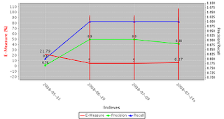
As we can see from the chart above, both recall and precision increased initially from the baseline index, and the E-Measure came down from 21.79 to 5, but then some algorithm change between 2008-07-09 and 2008-07-24x caused a slight decrease in the precision and a slight uptick in the E-Measure. I think automated search quality metrics such as these can be quite useful as an early warning system for unexpected side effects caused by some algorithm change, as well as a way to measure how a change or set of changes affect the overall search quality.