Searching for Answer Candidate Passages with Solr and Anserini

I just got back from our company's internal Search Summit at our offices at Raleigh, NC -- the conference is in its third year, and it has grown quite a bit from its humble beginnings. We even have our own conference sticker! The conference was 1 day of multi-track workshops, and two days of single track presentations. Our Labs team conducted a workshop on Bidirectional Encoder Representations from Transformers (or BERT), and I presented my results on BERT based Open Domain Question Answering.

Our BERT based Question Answering pipeline is inspired by the End-to-end Open-Domain Question Answering with BERTSerini paper from Prof Jimmy Lin's team from the University of Waterloo. We are using our own content from ScienceDirect, and we have been trying BERT, pre-trained variants such as BioBERT and SciBERT, and other models such as XLNet and AllenNLP BiDAF, fine tuned with SQuAD 1.1 and 2.0 datasets, and we are using the pipeline variants to answer our own set of questions in the scientific domain. Overall, we have gotten best results from SciBERT+SQuAD 1.1, but we are looking at fine-tuning with SQuAD 2.0 to see if we can get additional signal from when the model abstains from answering.

The figure below shows the BERTSerini pipeline (as described in the BERTSerini paper). In this post, I want to describe the Anserini Retriever component and our implementation of it as a Solr plugin. The Anserini Retriever is an open source IR toolkit described in Anserini: Enabling the Use of Lucene for Information Retrieval Research. It was originally built as a way to experiment with running things like TREC benchmarks, as described in Toward Reproducible Baselines: The Open-Source IR Reproducibility Challenge. It implements a pluggable strategy for handling question style queries against a Lucene index. The code for the Anserini project is available at castorini/anserini on Github.

Functionally, the Anserini retriever component takes as input a string representing a question, and returns a set of results that can be used as candidate passages by the Question Answering module. The pipeline consists of two steps -- query expansion and results reranking. Anserini offers multiple ways to do each step, allowing the caller to mix and match these strategies to create customized search pipelines. It also offers multiple pluggable similarity strategies, most commonly used of which seem to be BM25 (default similarity for Lucene and its derivative platforms nowadays) and QL (Query Likelihood). The question is parsed by the query expansion steps, and sent to the index, which I will call query A. Results from query A are then reranked -- the reranking is really another (filtered) query to the index, which I will call query B.

Query Expansion strategies include the Bag of Words (BoW), and the Sequential Dependency Model (SDM). Bag of words is fairly self explanatory, its just an OR query of all the tokens in the query, after stopwording, and optionally synonym expansion. SDM is only slightly more complex, it is a weighted query with three main clauses. The first clause is a Bag of Words. The second clause is an OR query of neighboring bigram tokens where proximity and order are both important, and the third clause is an OR query of neighboring bigram tokens where proximity is relaxed and order is not important. The three clauses are weighted in a compound OR query, default weights are (0.85, 0.1, 0.05).

The query (Query A) is sent to the index, which will return results. We take the top K results (configurable, we use K=50 as our default) and send it to the result reranking step. Anserini provides three pluggable reranking algorithms. They are RM3 (Relevance Model 3), Axiomatic, and Identity. RM3 computes feature vectors for query terms and the results from query A. Feature vectors for the results come from the top fbTerms (default 10) from each of the top fbDocs (default 10) documents in the result set. Query vectors and result vectors are interpolated using a multiplier alpha (default 0.5), and resulting top scoring terms are used to construct Query B as a weighted OR query, where the weights for each term is the score computed for it. The Axiomatic strategy is similar, except it uses a mix of the top rerankCutoff results from query A, and a random set of non-results to improve recall. It uses Mutual Information (MI) between query terms in the query and results to compute the top results. As with RM3, Query B for Axiomatic is a weighted OR query consisting of terms with highest MI and the corresponding weights are the MI values for the term. The Identity strategy, as the name suggests, is a no-op passthrough, which passes the output of Query A unchanged. It can be useful for debugging (in a sense "turning-off" reranking), or when the results of Query A produce sufficiently good candidates for question answering. Finally, since Query B is its own separate query, in order to ensure that it behaves as a reranker, we want to restrict the documents returned to those returned in the top rerankedCutoff documents from Query A. In the Solr plugin, we have implemented that as a docID filter on top results of Query A that is added to Query B.

Pluggable similarities is probably a bit of a misnomer. Way back, Lucene offered a single similarity implementation -- a variant of TF-IDF. Later they started offering BM25 as an alternative, and since Lucene 7.x (I believe), BM25 has become the default Similarity implementation. However, probably as a result of the changes needed to accommodate BM25, it became easier to add newer similarity implementations, and recent versions of Lucene offer a large variety of them, as you can see from the Javadocs for Lucene 8 Similarity. However, similarities are associated with index fields, so a pluggable similarity will only work if you indexed your field with the appropriate similarity in the first place. Anserini offers quite a few similarity implementations, corresponding to the different similarities available in Lucene. However, we noticed that in our case, we just needed BM25 and QL (Query Likelihood, corresponding to Lucene's LMDirichletSimilarity), so our Solr plugin just offers these two.

When I set out to implement the BERTSerini pipeline, my original thought was to leverage the Lucene code directly. However, I decided against it for a number of reasons. First, the scripts I saw in their repository suggested that the primary use case is running large benchmarks with different parameters in batch mode, whereas my use case (at least initially) was more interactive. Second, our index is fairly large, consisting of 4000 books from Science Direct, which translates to approximately 42 million records (paragraphs), and takes up 150 GB (approx) disk space, so we are constrained to build it on a cloud provider's machine (AWS in our case). With Lucene, the only way to "look inside" is Luke, which is harder to forward to your local machine over SSH, compared to forwarding HTTP. For these reasons I decided on using Solr as my indexing platform, and implementing the necessary search functionality as a Solr plugin.

Once I understood the functionality Anserini offered, it took just 2-3 days to implement the plugin and access it from inside a rudimentary web application. The figure below shows the candidate passages for a question that should be familiar to many readers of this blog -- How is market basket analysis related to collaborative filtering? If you look at the top 3 (visible) paragraphs returned, they seem like pretty good candidate passages. Overall, the (BM25 + BoW + RM3) strategy seems to return good passages for question answering.

While the plugin is currently usable as-is, i.e., it is responsive and produces good results, the code relies exclusively in copying functionality (and sometimes chunks of code) from the Anserini codebase rather than using Anserini as a library. In fact, the initial implementation (in the "master" branch) does not have any dependencies on the Anserini JAR. For long term viability, it makes sense to have the plugin be dependent on Anserini. I am currently working with Prof Lin to make that happen, and some partially working code is available to do this in the branch "b_anserini_deps".

The code for the Solr plugin (and documentation on how to install and use it) can be found in the elsevierlabs-os/anserini-solr-plugin repository on Github. My employer (Elsevier, Inc.) open sourced the software so we could (a) make it more robust as described above, in consultation with Prof Lin's team, and (b) provide a tool for Solr users interested in exposing the awesome candidate passage generation for question answering functionality provided by Anserini.

If you are working in this space and are looking for a good tool to extract candidate passages from questions, I think you will find the Solr plugin very useful. If you end up using it, please let us know what you think, including how it could be improved.

Trip Report (sort of): RELX Search Summit 2018

Last week, I was at our London office attending the RELX Search Summit. The RELX Group is the parent company that includes my employer (Elsevier) as well as LexisNexis, LexisNexis Risk Solutions and Reed Exhibitions, among others. The event was organized by our Search Guild, an unofficial special interest group of search professionals from all these companies. As you can imagine, search is something of a big deal at both LexisNexis and Elsevier, given several large, well known search platforms such as Lexis Advance, ScienceDirect, Scopus and Clinical Key.

There were quite a few interesting presentations at the Search Summit, some of which I thought was quite groundbreaking from an applied research point of view. I was going to write up a trip report for that when I realized that at least some of the talks probably represented competitive information that would not be appropriate for a public forum. Besides, it is very likely that it would of limited interest anyway. So I decided to write this post only about the two presentations that I did at the Summit. Neither of them are groundbreaking, but I think it might be interesting for most people in general. Hopefully you think so too.

The first presentation was a 3 hour tutorial session around Content Engineering. The theme I wanted to explore was how to identify keywords in text using various unsupervised and supervised techniques, and how this can improve search. As you know, my last job revolved around search driven by a medical ontology, where the ontology was painstakingly hand-curated by a team of doctors, nurses and pharmacists over a span of several years.

Having an ontology makes quite a few things much easier. (It also makes several things much harder, but we won't dwell on that here). However, the use case I was trying to replicate was where you have the content to search, but no ontology to help you with it. Could we, using a variety of rule-based, statistical and machine learning techniques, identify phrases that represent key ideas in the text, similar to concepts in our ontology? And how does this help with search?

The dataset I used was the NIPS (Neural Information Processing Systems) conference papers from 1987 to 2017. The hope was that I would learn something about the cool techniques and algorithms that show up at NIPS, just by having to look at the text to debug problems, although it didn't quite work out the way I had hoped. I demonstrate a variety of techniques such as LLR (statistical), RAKE (rule based) and MAUI (machine learning based), as well as using Stanford and SpaCy NER models, and duplicate keyword detection and removal using SimHash and Dedupe. In addition, I also demonstrate how to do dimensionality reduction using various techniques (PCA, Topic Modeling, NMF, word vectors) and how they can be used to enhance the search experience. In addition, another point I was trying to make was that there is plently of third party open source tools available to do this job without significant investment in coding.

All the techniques listed above are demonstrated using Jupyter notebooks. In addition, I built a little Flask based web application that showed these techniques in action against a Solr 7.3 index containing the NIPS papers. The web application demonstrates techniques both on the query parsing side where we rewrite queries in various ways to utilize the information available, as well as on the content side, where the additional information is used to suggest documents like the one being viewed, or make personalized reading recommendations based on the collection of documents read already.

The presentation slides, the notebooks and the web application can all be found in my sujitpal/content-engineering-tutorial project on Github. Several new ideas were suggested by participants during the tutorial, since many of them had been looking at similar ideas already, so it morphed into a nice interactive workshop style discussion. I hope to add them in as I find time.

My second presentation was around Learning to Rank (LTR) basics. I had recently become interested in LTR following my visit to the Haystack Search Relevancy conference earlier this year, coupled with a chance discovery that a content-based recommender system I was working to help improve had around 40,000 labeled query document pairs, which could be used to improve the quality of recommendations.

The dataset I chose for this presentation was The Movie DataBase (TMDB), a collection of 45,000 movies, 20 genres and 31,000 unique keywords. The idea was to see if I could teach a RankLib LambdaMART model the ordering given by the rating field on a 10 point continuous scale. In a sense, the approach is similar to this LTR article using scikit-learn by Alfredo Motta. Most LTR datasets just give you the features dataset in LETOR format to train your ML models, so you can't actually do the full end-to-end pipeline.

In any case, the presentation starts off with a little bit of historical context, talks about different kinds of LTR models (pointwise, pairwise and listwise), some common algorithms that people tend to use, some advice to keep in mind when considering building an LTR model, ideas for features, the LETOR data format, etc. Most of the meat of the presentation is the creation of an LTR model using the Solr 7.4 and Elasticsearch 6.3.1 plugins, as well for a hypothetical indexer with no LTR support (I used Solr, but did the feature generation outside the indexer). I was hoping to cover at least one of the case studies but ran into technical difficulties (my fault, I should have listened to the organizers when they said to put everything in the slides).

Essentially, the methodology is similar for either of the 3 case studies, the main differences are in syntax (for Solr vs Elasticsearch). First we need a set of queries with a ranked list of documents for each. I used the ratings to create categorical query-document labels on a 5 point scale as explained earlier.

Once the data is loaded, the first step is to define the features to Solr and Elasticsearch - features are specified as function queries. We then generate the feature values from Solr or Elasticsearch by running the queries against these function queries and writing the features into a file in LETOR format. The reason we use the index is mostly to generate the query-document similarity features. For a system without LTR support, this can be done less efficiently outside the index as well.

The LETOR format was originally used by the LTR model suite RankLib (provides 8 different LTR models), and has since been adopted by most other third party LTR models. I trained a RankLib LambdaMART model for all 3 cases. Model training has to happen using third party algorithms, of which RankLib is one. The output of RankLib is an XML file whose format varies depending on what kind of model it represents. For a linear model, it is just a set of coefficients for each of the features defined. For RankNet, a neural network, it is a weight matrix that transforms the incoming features into a set of rank probabilities. For LambdaMART, which is a forest of decision trees, it is a set of trees, each with splits defined for various levels.

Once the model is trained, it has to be uploaded to Solr or Elasticsearch. Solr needs the model to be specified in JSON format, so you need to write some code to convert the XML to JSON, while Elasticsearch will accept the XML definition of the trained model without any conversion. You can now use the rerank functionality in Solr or Elasticsearch to rerank the top slice of a base query. For indexers that don't have LTR support, you will have to generate the search results, extract and rerank the top slice using your trained model, and add it back into the search results yourself.

Notebooks and scripts describing each of the case studies as well the presentation slides can be found in my sujitpal/ltr-examples repository on Github. My main objective here was to understand how to "do" LTR using Solr and Elasticsearch, so I didn't spend much time trying to improve results. Perhaps if I can find a bigger labeled dataset to play with, I might revisit this project and try to evaluate each platform in more detail, would appreciate suggestions if you know of any such datasets. Note that standard LTR datasets such as MSLR-WEB10K just provide the features in LETOR format, so it is all about the part where you train and evaluate the LTR model, nothing to do with showing the results on the search index. What I am looking for is a dataset with labeled query-document pairs.

That's all I have for today. This week I am at RecSys 2018 at Vancouver, hoping to learn more about recommendation systems from the very best in the field, and meet others working in the recommendation space. Do ping me if you are here as well, would be nice to meet face to face.

Scoring token distance in Lucene sloppy queries

Lucene (and Lucene based search platforms such as Solr and ElasticSearch) has the concept of slop for inexact phrase queries, which specifies how loose the phrase matching can be. For example, "four seven" would not match a document containing the Gettysburg Address, but "four seven"~2 or "seven four"~3 would. Here the slop is the number of token transpositions it would take for the query string to match the target string.

This was all I knew about slop for a long time and I never had a need to know beyond this. Recently, however, I was working with some people whose had a background in other search engines, and they raised the question, that given two documents like this:

• Four of five fathers don't know..."
• Four score and seven years ago, our fathers brought forth on this continent...

and a query "four fathers"~20, which one of these would score higher and by how much? My understanding was that slop is merely a filtering mechanism and both results would show up in no particular order. Turns out this is not quite true - while slop does serve to filter the results, the distance between the tokens does influence the final scores. I would have chalked it up to ignorance on my part and moved on, but a quick poll among some of my Lucene programmer colleagues revealed that this is something most people hadn't really thought about, so I thought it may be useful to write about it. Hence this post.

In order to investigate the variation of score with token distance, I set up the following simple experiment. I built a set of "documents", each with exactly 42 1-character "words" consisting of the letters a-j repeated 4 times. The first word in each document was x and another character y was put into the second, third, fourth, etc token positions. So my "documents" looked something like this:

1 2 3 4

x y a b c d ... x a y b c d ... x a b y c d ... ...

To build this corpus of documents, I wrote this little Python script to build an array of JSON documents like so:

1 2 3 4 5 6 7 8 9 10 11 12 13 14

import string first_10 = string.lowercase[0:10] doc_tpl = first_10[0:1] + 'x' + first_10[1:] + first_10*3 doc_id = 0 print("[") for i in range(len(doc_tpl)-2): doc = doc_tpl[0:i+2] + 'y' + doc_tpl[i+2:] doc_title = " ".join([c for c in doc]) print("{\"id\":\"%s\", \"title\":\"%s\"}," % (doc_id, doc_title)) doc_id = doc_id + 1 print("]")

This is sent to Solr's update handler using a curl command like so:

1 2	curl "http://localhost:8983/solr/update/json?commit=true" \ -H "Content-type:application/json" --data-binary @test_data.json

We then send a single sloppy query "x y"~20 to Solr and graph the resulting scores. I then use Scipy's curve_fit command to fit the points to a formula I derived by looking at the explain output and the code (described after the graph).

1 2 3 4 5 6 7 8 9 10 11 12 13 14 15 16 17 18 19 20 21 22 23 24 25 26 27 28 29 30 31 32 33 34 35 36 37 38 39 40 41 42 43 44 45 46 47

from __future__ import division import urllib2 import urllib import json import matplotlib.pyplot as plt import numpy as np from scipy.optimize import curve_fit import math def proximity_score(x, a, b): return a + b / np.power(x + 1, 0.5) url = "http://localhost:8983/solr/collection1/select" urlparams = { "q": "*:*", "wt": "json", "rows": "0", "fl": "id,score" } conn = urllib2.urlopen(url + "?" + urllib.urlencode(urlparams)) response = json.load(conn) count = response["response"]["numFound"] conn.close() urlparams["q"] = "\"x y\"~20" urlparams["rows"] = str(count) conn = urllib2.urlopen(url + "?" + urllib.urlencode(urlparams)) response = json.load(conn) xs = [] ys = [] for doc in response["response"]["docs"]: xs.append(int(doc["id"])) ys.append(float(doc["score"])) conn.close() axs = np.array(xs) ays = np.array(ys) plt.plot(axs, ays, 'bo', label="Actual") popt, pcov = curve_fit(proximity_score, axs, ays) print popt plt.plot(axs, proximity_score(axs, *popt), 'r--', linewidth=1.5, label="Fitted") plt.xlabel("Distance between tokens") plt.ylabel("Score") plt.legend() plt.show()

This gives us the chart shown below. The blue points are the actual scores returned for each record with the specified token distances between the tokens x and y, and the red dotted line is the curve given by:

1	score = 9.96e-10 + (0.25 / math.sqrt(dist + 1))

Here the intercept term is almost zero, and the 0.25 in the numerator is an artifact of the other parameters in the experiment. The takeaway is that scores vary as the inverse of the square root of the between token distance for sloppy queries, all other things being constant.

I had initially tried to plot an exponential curve, but it didn't match as well as this one. So I started looking at the explain output for clues. Here is the explain for the top 3 results, formatted for readbility.

1 2 3 4 5 6 7 8 9 10 11 12 13 14 15 16 17 18 19 20 21 22 23 24 25 26 27 28

0: 0.24367055 = (MATCH) weight(text:"x y"~20 in 0) [DefaultSimilarity], result of: 0.24367055 = fieldWeight in 0, product of: 1.0 = tf(freq=1.0), with freq of: 1.0 = phraseFreq=1.0 1.9493644 = idf(), sum of: 0.9746822 = idf(docFreq=39, maxDocs=39) 0.9746822 = idf(docFreq=39, maxDocs=39) 0.125 = fieldNorm(doc=0), 1: 0.1723011 = (MATCH) weight(text:"x y"~20 in 1) [DefaultSimilarity], result of: 0.1723011 = fieldWeight in 1, product of: 0.70710677 = tf(freq=0.5), with freq of: 0.5 = phraseFreq=0.5 1.9493644 = idf(), sum of: 0.9746822 = idf(docFreq=39, maxDocs=39) 0.9746822 = idf(docFreq=39, maxDocs=39) 0.125 = fieldNorm(doc=1), 2: 0.14068326 = (MATCH) weight(text:"x y"~20 in 2) [DefaultSimilarity], result of: 0.14068326 = fieldWeight in 2, product of: 0.57735026 = tf(freq=0.33333334), with freq of: 0.33333334 = phraseFreq=0.33333334 1.9493644 = idf(), sum of: 0.9746822 = idf(docFreq=39, maxDocs=39) 0.9746822 = idf(docFreq=39, maxDocs=39) 0.125 = fieldNorm(doc=2)\n", ...

On inspecting the output, I realized that the variation was happing in the phraseFreq line, falling off as (1, 0.5, 0.33, ...), ie by the inverse of the distance. Looking at the code for DefaultSimilarity, it looks like phraseFreq contributes the square root of itself plus 1 to the score via tf(phraseFreq) in the line immediately above.

This is all I have for this week. Hopefully I was able to share something you didn't know through this experiment.

Exploring Solr GeoSearch capabilities

At my previous job at Healthline, my use of Lucene and Solr were focused on its text analysis and search capabilities. While there have been various initiatives involving use of Solr's Geosearch (Spatial) capabilities, primarily in applications that involved finding medical providers (doctors, hospitals, etc), these were invariably done by others in the group. As a result, I have remained largely ignorant of what is possible using Solr's Spatial functionality. The ignorance has come back to bite me at least once recently, when I had to commit to a level of effort estimate on a project that had a Geosearch component.

I had some time last week so I decided to explore Solr's Spatial capabilities. For data, I used the free 500 US addresses dataset from Brian Dunning's website, available in comma-separated (CSV) with quoted string fields. I didn't want to use a full-blown CSV reader, so I opened it with OpenOffice Calc and converted it to tab-separated (TSV). I then took the addresses and annotated them with latitude and longitude using Google's Geocoding API. I then populated a Solr index with the annotated data, and ran some Spatial queries to understand the possibilities.

Here is the code to read the CSV file, and for each record, call Google's Geocoding API and annotate the record with the latitude and longitude. One thing to realize is that the annotation is only as good as your data. The Geocoding API is basically doing an address search - if you look at the output, you will see that it is breaking down the address into various components and trying to do a best match against various internal fields, and coming up with a best guess as to the latitude-longitude component. So in some cases, the latitude-longitude pair returned is not that of the address but of the closest matched point in the Geocoding API's database. Also some addresses cannot be mapped to a LatLon pair, they are given a LatLon of (0,0).

1 2 3 4 5 6 7 8 9 10 11 12 13 14 15 16 17 18 19 20 21 22 23 24 25 26 27 28 29 30 31 32 33 34 35 36 37 38 39 40 41 42 43 44 45 46 47 48 49 50 51 52 53 54 55 56 57 58 59 60 61 62 63 64 65 66

// Source: src/main/scala/com/mycompany/solr4extras/geo/LatLonAnnotator.scala package com.mycompany.solr4extras.geo import java.io.File import java.io.FileWriter import java.io.PrintWriter import java.net.URLEncoder import scala.io.Source import org.codehaus.jackson.map.ObjectMapper class LatLonAnnotator { val googleApiKey = "secret" val geocodeServer = "https://maps.googleapis.com/maps/api/geocode/json" val objectMapper = new ObjectMapper() def annotate(addr: String): (Double,Double) = { val params = Map( ("address", URLEncoder.encode(addr)), ("key", googleApiKey)) val url = geocodeServer + "?" + params.map(kv => kv._1 + "=" + kv._2) .mkString("&") val json = Source.fromURL(url).mkString val root = objectMapper.readTree(json) try { val location = root.path("results").get(0) .path("geometry").path("location") val lat = location.path("lat").asDouble val lon = location.path("lng").asDouble (lat, lon) } catch { case e: Exception => (0.0D, 0.0D) } } def batchAnnotate(infile: File, outfile: File): Unit = { val writer = new PrintWriter(new FileWriter(outfile), true) val lines = Source.fromFile(infile) .getLines() .filter(line => !line.startsWith("first_name")) .foreach(line => { val cols = line.split("\t") val fname = cols(0) val lname = cols(1) val company = cols(2) val address = cols(3) val city = cols(4) val state = cols(6) val zip = cols(7) val apiAddress = List(address, city, state) .mkString(", ") + " " + zip Console.println(apiAddress) val latlon = annotate(apiAddress) writer.println(List(fname, lname, company, address, city, state, zip, latlon._1, latlon._2) .mkString("\t")) Thread.sleep(1000) // sleep 1s between calls to Google API }) writer.flush() writer.close() } }

You will need a Google API key for the Geocoding API. The free service is quite generous - they give you 5,000 lookups per day and throttle it upto 5 requests/s. Because my dataset was so small, I was able to test my code and run two full runs within a single day's limit. Key generation is simple, but I found navigating the Google developer site kind of non-intuitive - you can find the information about generating and using your keys here.

I wanted to see the coverage of these 500 US addresses, so I wrote a small R script to do this (with lots of help from this page). Here is the R script and the output. As you can see, there is a nice concentration of addresses around the New York/New Jersey/Washington DC area, which is what we will use for our testing.

1 2 3 4 5 6 7 8 9 10 11 12 13 14 15 16

# Source: viz.R library(maps) png("addr_dist.png") map("state", interior=F) map("state", boundary=F, col="gray", add=T) data = read.csv("us-cities-annotated.csv", sep="\t", col.names=c("fname", "lname", "company", "address", "city", "state", "zip", "lat", "lon")) data.clean = data[!(data$lat==0 & data$lon==0), ] points(data.clean$lon, data.clean$lat, pch=19, col="red", cex=0.5) dev.off()

The indexing code is fairly straightforward, we leverage Solr's dynamic fields to set most of our address fields into either text or string fields. The latitude longitude pair we retrieved from the Geocoding API go into a special field type called LatLonType as a comma-separated pair.

1 2 3 4 5 6 7 8 9 10 11 12 13 14 15 16 17 18 19 20 21 22 23 24 25 26 27 28 29 30 31 32 33 34 35 36 37 38 39

// Source: src/main/scala/com/mycompany/solr4extras/geo/LatLonIndexer.scala package com.mycompany.solr4extras.geo import java.io.File import java.util.concurrent.atomic.AtomicInteger import scala.io.Source import org.apache.solr.client.solrj.impl.HttpSolrServer import org.apache.solr.common.SolrInputDocument class LatLonIndexer { val solrUrl = "http://localhost:8983/solr/collection1" val infile = new File("src/main/resources/us-cities-annotated.csv") def buildIndex(): Unit = { val solr = new HttpSolrServer(solrUrl) val ctr = new AtomicInteger(0) Source.fromFile(infile).getLines() .foreach(line => { val doc = new SolrInputDocument() val cols = line.split("\t") doc.addField("id", ctr.addAndGet(1)) doc.addField("firstname_s", cols(0)) doc.addField("lastname_s", cols(1)) doc.addField("company_t", cols(2)) doc.addField("street_t", cols(3)) doc.addField("city_s", cols(4)) doc.addField("state_s", cols(5)) doc.addField("zip_s", cols(6)) doc.addField("latlon_p", List(cols(7), cols(8)).mkString(",")) solr.add(doc) }) solr.commit() solr.shutdown() } }

Finally, we now leverage Solr's Spatial capabilities as described on its wiki page. Here is the code for the searcher.

1 2 3 4 5 6 7 8 9 10 11 12 13 14 15 16 17 18 19 20 21 22 23 24 25 26 27 28 29 30 31 32 33 34 35 36 37 38 39 40 41 42 43 44 45 46 47 48 49 50 51 52 53 54 55 56 57 58 59 60 61 62 63 64 65 66

// Source: src/main/scala/com/mycompany/solr4extras/geo/LatLonSearcher.scala package com.mycompany.solr4extras.geo import org.apache.solr.client.solrj.SolrQuery import org.apache.solr.client.solrj.impl.HttpSolrServer import org.apache.solr.common.SolrDocument import scala.collection.JavaConversions._ class LatLonSearcher { val solr = new HttpSolrServer("http://localhost:8983/solr/collection1") def findWithinByGeofilt(p: Point, dkm: Double, sort: Boolean, nearestFirst: Boolean): List[LatLonDoc] = findWithin("geofilt", p, dkm, sort, nearestFirst) def findWithinByBbox(p: Point, dkm: Double, sort: Boolean, nearestFirst: Boolean):List[LatLonDoc] = findWithin("bbox", p, dkm, sort, nearestFirst) def findWithin(method: String, p: Point, dkm: Double, sort: Boolean, nearestFirst: Boolean): List[LatLonDoc] = { val query = new SolrQuery() query.setQuery("*:*") query.setFields("*") query.setFilterQueries("{!%s}".format(method)) query.set("pt", "%.2f,%.2f".format(p.x, p.y)) query.set("d", dkm.toString) query.set("sfield", "latlon_p") if (sort) { query.set("sort", "geodist() %s" .format(if (nearestFirst) "asc" else "desc")) query.setFields("*,_dist_:geodist()") } val resp = solr.query(query) resp.getResults() .map(doc => getLatLonDocument(doc)) .toList } def getLatLonDocument(sdoc: SolrDocument): LatLonDoc = { val latlon = sdoc.getFieldValue("latlon_p") .asInstanceOf[String] .split(",") .map(_.toDouble) val dist = if (sdoc.getFieldValue("_dist_") != null) sdoc.getFieldValue("_dist_").asInstanceOf[Double] else 0.0D LatLonDoc(sdoc.getFieldValue("firstname_s").asInstanceOf[String], sdoc.getFieldValue("lastname_s").asInstanceOf[String], sdoc.getFieldValue("company_t").asInstanceOf[String], sdoc.getFieldValue("street_t").asInstanceOf[String], sdoc.getFieldValue("city_s").asInstanceOf[String], sdoc.getFieldValue("state_s").asInstanceOf[String], sdoc.getFieldValue("zip_s").asInstanceOf[String], Point(latlon(0), latlon(1)), dist) } } case class Point(x: Double, y: Double) case class LatLonDoc(fname: String, lname: String, company: String, street: String, city: String, state: String, zip: String, location: Point, dist: Double)

The main method the searcher code above exposes is the findWithin() method. You can specify one of two methods for finding LatLon points within a certain distance d (in kilometers) from a Point p. The two methods are geofilt and bbox - geofilt finds points within a circle and bbox finds points within a square (bounding box). The bbox method is slightly looser than the geofilt method (ie may return points farther away than d km from p), but is less heavier performance-wise. The findWithin() method also supports sorting by distance, using the geodist() function. Internally, these are implemented as function queries.

Of course, provider search is generally more than just searching by LatLon. The query as implemented in the code above will most likely only be triggered from the value of the entered zipcode, where each zipcode is mapped to a central LatLon point within it using data like this. In reality, provider search would include searching by provider's name, specialties, languages spoken, etc. The code above puts the LatLon search into the filter query (fq) portion, so we could add in queries for other parts of the lookup into either the main query (q) or additional clauses in the fq. There are other use cases one could explore, such as faceting by distance (see the wiki page above).

1 2 3 4 5 6 7 8 9 10 11 12 13 14 15 16 17 18 19 20 21 22 23 24 25 26 27 28 29 30 31 32 33 34 35 36 37 38 39 40 41 42 43 44 45 46

// Source: src/test/scala/com/mycompany/solr4extras/geo/LatLonSearcherTest.scala package com.mycompany.solr4extras.geo import org.junit.Test import org.junit.Assert class LatLonSearcherTest { val dcLocation = Point(38.89, -77.04) val searcher = new LatLonSearcher() @Test def testFindWithinByGeofilt(): Unit = { val results = searcher.findWithin( "geofilt", dcLocation, 50, false, false) val neighborStates = results.map(_.state).toSet Assert.assertEquals(9, results.size) Assert.assertEquals(2, neighborStates.size) Assert.assertTrue(neighborStates.contains("MD") && neighborStates.contains("VA")) } @Test def testFindWithinByBbox(): Unit = { val results = searcher.findWithin( "bbox", dcLocation, 50, false, false) val neighborStates = results.map(_.state).toSet Assert.assertEquals(10, results.size) Assert.assertEquals(2, neighborStates.size) Assert.assertTrue(neighborStates.contains("MD") && neighborStates.contains("VA")) } @Test def testSortByDistance(): Unit = { val results = searcher.findWithin( "bbox", dcLocation, 50, true, true) Assert.assertTrue(results.head.dist < results.last.dist) val formattedResults = results .map(result => "%s, %s %s %s (%.2f km)" .format(result.street, result.city, result.state, result.zip, result.dist)) .foreach(Console.println(_)) } }

The code above shows the test case we use to exercise our LatLonSearcher code. The first and second tests show how to call the findWithin() method with the "geofilt" and "bbox" methods. No sorting is performed on the distance between the query point (dcLocation, a point within the Washington DC metro area) and the target addresses. The first test returns 9 results and the second test returns 10, lending credence to the assertion that bbox is looser than geofilt. We also see that the results have addresses in Virginia and Maryland, two states that border Washington DC. The third test illustrates calling findWithin() using the bbox method and with results sorted by distance (closest first). Here are the results of this test - as you can see, there are 10 results, the last of which is outside the 50km radius (because of bbox).

1 2 3 4 5 6 7 8 9 10

64 5th Ave #1153, Mc Lean VA 22102 (5.79 km) 9506 Edgemore Ave, Bladensburg MD 20710 (12.45 km) 5 Cabot Rd, Mc Lean VA 22102 (12.84 km) 94 Chase Rd, Hyattsville MD 20785 (14.28 km) 747 Leonis Blvd, Annandale VA 22003 (14.73 km) 47857 Coney Island Ave, Clinton MD 20735 (20.56 km) 48 Lenox St, Fairfax VA 22030 (21.70 km) 3387 Ryan Dr, Hanover MD 21076 (43.49 km) 2853 S Central Expy, Glen Burnie MD 21061 (46.93 km) 2 W Scyene Rd #3, Baltimore MD 21217 (57.92 km)

And this is all I have for today. For those of you who have worked with Solr Spatial before, this post is probably going to be pretty basic, but for those of you who haven't, I hope that this gives a quick high level overview of what you can do with it. If you need it, the (Scala) code for this post is available on my project on GitHub.

More Scala Web Development with Spring and JSTL

Continuing on from my previous blog post, where I describe the setup and some initial work to build a custom Business Intelligence (BI) tool around anonymized Medicare data, using Solr, Scala, Spring and JSTL. In this post, I will cover the remainder of the application, but unlike most of my other posts, I won't include any code. Instead, I will describe the tool from a (mostly) user-centric perspective, describing what you can do with it, and taking short detours to address the how. All the code for this project is available on GitHub, along with instructions on how to run the tool locally.

Population View

I left off last week with a single page application, the Population Demographics view. On this page, we report the distribution of members across attributes such as gender, age, ethnicity, state of residence and diseases (a member can have zero or more diseases). Each distribution is reported as a bar chart and a table in which the user is able to select one or more attribute values. Shown below is the report for the Age distribution.

Somewhat unsurprisingly, the majority of members appear to be aged between 70 and 90. Similarly, if you look at the other attributes, you will find that members are 45% Male and 55% Female, and that the majority are White (83%). California, Florida, Texas and New York have the most members (9%, 7%, 5.8% and 5.7% respectively). The most frequently observed disease is Ischemic Heart Disease (IHD) at 19%, followed by Diabetes at 17% and Congestive Heart Failure (CHF) at 13%. Interesting information perhaps (at least to lay people like me), but probably not news for people who work in population health.

But what if you are interested in the disease profile for 30-50 year old men from California compared to the national average? From the screenshots below, the younger cohort from CA (left) appears to be proportionally more prone to Depression and less prone to Cancer.


Or imagine you wanted to know how the ethnic distribution of members from California has changed in recent years. The screenshot on the right shows the ethnic distribution of members 30-40 years old and the one on the left shows the distribution for ages 40 and up. As you can see, California has become more diverse in recent years, at least in terms of Medicare members.


The functionality described above were implemented with Solr's Faceted Search. In all but Age, the attributes (Gender, Ethnicity, State and Disease) were the facet fields. In case of Age, we sent two initial Sort queries to find the minimum and maximum dates of birth, then partitioned the range into 10 bins, building the facets using date range queries. All the Solr code can be found in SolrService.scala.

Mortality View

Once you have selected a subpopulation in this manner, you can look at various other things. For a somewhat morbid example, you can look at the distribution of mortality rates for various diseases. Here is the distribution of ages of death for members who had some form of heart disease.

A subset of member records had a date of death populated. I found this after populating the index (populating the index took a little over a day for me), so I used Solr's partial update feature (see MortalityUpdater.scala) to compute a new age_at_death field from the birth and death dates and update this field into the index. From that point on it was two queries to get the max and min ages, partitioning the range and building a set of range facet queries on this field.

Codes View

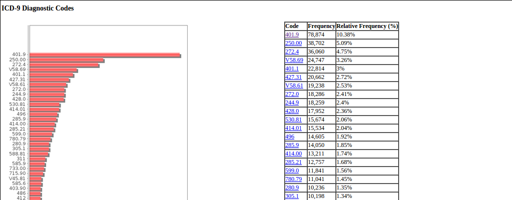
Another way to look at a selected subpopulation is as a distribution of medical codes. Three types of codes are mentioned in the claims - the ICD-9 diagnostic codes, the ICD-9 procedure codes and the HCPCS codes. Below we show the top ICD-9 diagnostic codes for 30-60 year old Male Californians with heart disease (IHD, CHF and Stroke/TIA).

The top ICD-9 code 401.9 means Unspecified Essential Hypertension, aka High Blood Pressure, which seems to be a reasonable diagnosis for heart disease patients. It occurs 10% of the time across both types of claim - Inpatient and Outpatient. You can click on the codes to go to code lookup pages hosted by cms.gov, but if you are a company doing this for real, you would probably want to buy the code list and have the description show up beside the code without this extra step. The above results can also be filtered to show only Inpatient claims or Outpatient claims. You can also do similar analysis for the other two codes as well.

The chart and associated reports for the three codes were done using a single Solr FacetQuery with facet fields set to the three multivalued code fields, filtering by the population selection criteria.

Costs View

Similar to the Codes view, where we analyze the distribution of codes, in the costs view, we analyze the distribution of costs across claims. I decided to use the claim payment amount as the "cost" parameter. Here is the cost distribution for the same cohort as before.

As you can see, most of the claim payments are under $1,000 and a small number of much higher values. The mean is $1,090 and standard deviation is $3,750. For a more interesting look, we can drill down to the range $0-$1,000.

This shows peaks at specific amounts - I suspect that these may be standard negotiated rates, but I could be wrong. For the implementation details, once again we compute the minimum and maximum claim payment amount for the selected cohort, then split up the range into 50 buckets, then execute the corresponding 50 facet queries (its a single request) using Solr's Facet Query functionality. The descriptive statistics box with Min, Max, Mean, StdDev, etc are from Solr's StatComponent.

Correlations View

Often it is instructive to see how a pair of parameters vary with each other. Correlations are often modeled with scatter plots, here we do this using a bubble chart with actual values for categorical variables like gender, ethnicity, state and comorbidity, and ranges for continuous variables like age. Here is a plot of the incidence of specific diseases over various age ranges, across the entire dataset.

Predictably, the incidence of various diseases seems to be highest in the 70-90 age range, although some of this is also the effect of higher number of members in this age group. Other correlations charts can be built as shown in the form above the chart above. Also you can also run each on population subsets, as shown below for our cohort of 30-60 year old male Californians with heart disease.

These bubble charts are backed by Solr Pivot Queries, a form of facet query where one can specify multiple dimensions of hierarchical facets (our example does two dimensions). This is true for all the facets except the ones that involve age. Since age is computed, it cannot reside in the index and therefore cannot participate in a facet query, so we simulate this by running multiple simple facet queries based on query facets and combining the results in code.

Patients View

The Patients View shows the actual member information for members in the selected cohort (based on what we have, since the data is anonymized). We order the patients by descending order of number of transactions, since the "interesting" patients from a data analyst's point of view are the ones with more transactions. For this, I added a new field num_io to each member record that counts the number of associated Inpatient and Outpatient claims, and sorted on that field. I could probably have used Solr's Join functionality but I had already denormalized the claim records to include the member data, and that was working better for me for the cohort filtering, so I decided not to. Here is the list of members for our 30-60 year old male Californians with heart disease cohort.

You could then select a particular patient and view the claim timeline, as shown in the example below. The chart across the top represents the claim amounts as a function of time (days since start on X-axis). The highlighted rows represent Inpatient claims and the others represent Outpatient claims.

Implementation wise, I used Solr's Solr's Deep paging feature to efficiently traverse the claim records from start to end (see IOCountUpdater.scala) and the partial update feature to update the num_io field. The search part is just simple filtering and sorting, we are not even using Lucene's query functionality here. In the first case (patient list), we are sorting by num_io and in the second case (patient timeline) we are sorting by claim date.

Charts

The charts in the application are built using the JFreeChart API. The ChartService.scala provides the services to draw 3 different types of charts - barchart, line and bubble. They are called from the chart() method in the ClaimController.scala, and the actual calls to it are made from JSPs via HTML img tags.

Nothing too fancy here, of course. The only reason I bring it up is that the data to plot is passed to the chart.html call as a URL-Encoded JSON Map object. Since the data is dynamically generated from a query, it can often be quite long and exceed the default length limit for HTTP GET URLs (8k chars for Tomcat and Jetty). To get around this, the container configuration needs to be tweaked to increase this limit (somewhat arbitarily to 64k chars). This is already done for the built-in Jetty container (via the custom jetty.xml, but if you want to do this on a standalone container, here are instructions for Jetty and Tomcat.

In retrospect, I should have used a List[(String,Double)] instead of a Map[String,Double], since the latter choice needs an additional sorting step inside the ChartService, but by the time it started hurting, I had already built a few charts, so I decided to just go with it and deal with it later.

Conclusion

Thats all I have today, hope you found it interesting. While the components that make up the tool are fairly commonplace, the tool can be used to slice and dice the data in interesting ways to derive intelligence out of this data and to find subpopulations of interest. In addition, (for me) it helped me play with some of the newer features of Solr 4.x with non-text data. In any case, its almost Thanksgiving, so for those of you in the US and Canada, Happy Thanksgiving, and for those of you not in the US or Canada, here's the link to Wikipedia :-).