Disambiguating SciSpacy + UMLS entities using the Viterbi algorithm

The SciSpacy project from AllenAI provides a language model trained on biomedical text, which can be used for Named Entity Recognition (NER) of biomedical entities using the standard SpaCy API. Unlike the entities found using SpaCy's language models (at least the English one), where entities have types such as PER, GEO, ORG, etc., SciSpacy entities have the single type ENTITY. In order to further classify them, SciSpacy provides Entity Linking (NEL) functionality through its integration with various ontology providers, such as the Unified Medical Language System (UMLS), Medical Subject Headings (MeSH), RxNorm, Gene Ontology (GO), and Human Phenotype Ontology (HPO). 

The NER and NEL processes are decoupled. The NER process finds candidate entity spans, and these spans are matched against the respective ontologies, which may result in the span matching zero or more ontology entries. All candidate span is then matched to all the matched entities. 

I tried annotating the COVID-19 Open Research Dataset (CORD-19) against UMLS using the SciSpacy integration described above, and I noticed significant ambiguity in the linking results. Specifically, annotating approximately 22 million sentences in the CORD-19 dataset results in 113 million candidate entity spans, which get linked to 166 million UMLS concepts, i.e., on average, each candidate span resolves to 1.5 UMLS concepts. However, the distribution is Zipfian, with approximately 46.87% entity spans resolving to a single concept, with a long tail of entity spans being linked to up to 67 UMLS concepts. 

In this post, I will describe a strategy to disambiguate the linked entities. Based on limited testing, this chooses the correct concept about 73% of the time. 

The strategy is based on the intuition that an ambiguously linked entity span is more likely to resolve to a concept that is closely related to concepts for the other non-ambiguously linked entity spans in the sentence. In other words, the best target label to choose for an ambiguous entity is the one that is semantically closest to the labels of other entities in the sentence. Or even more succintly, and with apologies to John Firth, an entity is known by the company it keeps. 

The NER and NEL processes provided by the SciSpacy library allows us to reduce a sentence to a collection of entity spans, each of which map to zero or more UMLS concepts. Each UMLS concept maps to one or more Semantic Types, which represent high level subject categories. So essentially, a sentence can be reduced to a graph of semantic type using the following steps. 

Consider the sentence below, the NER step identifies candidate spans that are indicated by highlights.

The fact that viral antigens could not be demonstrated with the used staining is not the result of antibodies present in the cat that already bound to these antigens and hinder binding of other antibodies.

The NEL step will attempt to match these spans against the UMLS ontology. Results for the matching are shown below. As noted earlier, each UMLS concept maps to one or more sematic types, and these are shown here as well.

   

Entity-ID	Entity Span	Concept-ID	Concept Primary Name	Semantic Type Code	Semantic Type Name
1	staining	C0487602	Staining method	T059	Laboratory Procedure
2	antibodies	C0003241	Antibodies	T116	Amino Acid, Peptide, or Protein
				T129	Immunologic Factor
3	cat	C0007450	Felis catus	T015	Mammal
		C0008169	Chloramphenicol O-Acetyltransferase	T116	Amino Acid, Peptide, or Protein
				T126	Enzyme
		C0325089	Family Felidae	T015	Mammal
		C1366498	Chloramphenicol Acetyl Transferase Gene	T028	Gene or Genome
4	antigens	C0003320	Antigens	T129	Immunologic Factor
5	binding	C1145667	Binding action	T052	Activity
		C1167622	Binding (Molecular Function)	T044	Molecular Function
6	antibodies	C0003241	Antibodies	T116	Amino Acid, Peptide, or Protein
				T129	Immunologic Factor

The sequence of entity spans, each mapped to one or more semantic type codes can be represented by a graph of semantic type nodes as shown below. Here, each vertical grouping corresponds to an entity position. The BOS node is a special node representing the beginning of the sequence. Based on our intuition above, entity disambiguation is now just a matter of finding the most likely path through the graph.

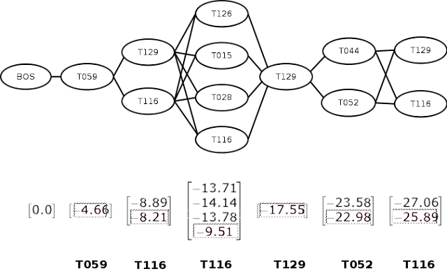
Of course, "most likely" implies that we need to know the probabilities for transitioning between semantic types. We can think of the graph as a Markov Chain, and consider the probability of each node in the graph as being determined only by its previous node. Fortunately, this information is already available as a result of the NER + NEL process for the entire CORD-19 dataset, where approximately half of the entity spans mapped unambiguously to a single UMLS concept. Most concepts map to a single semantic type, but in cases where they map to multiple, we consider them as separate records. We compute pairwise transition probabilities across semantic types for these unambiguously linked pairs across the CORD-19 dataset and create our transition matrix. In addition, we also create a matrix of emission probabilities that identify the probabilities of resolving to a concept given a semantic type. 

Using the transition probabilities, we can traverse each path in the graph from starting to ending position, computing the path probability as the product of transition probabilities (or for computational reasons, the sum of log-probabilities) of the edges. However, better methods exist, such as the Viterbi algorithm, which allows us to save on repeated computation of common edge sequences across multiple paths. This is what we used to compute the most likely path through our semantic type graph. 

The Viterbi algorithm consists of two phases -- forward and backward. In the forward phase, we move left to right, computing the log-probability of each transition at each step, as shown by the vectors below each position in the figure. When computing the transition from multiple nodes to a single node (such as the one from [T129, T116] to [T126], we compute for both paths and choose the maximum value. 

In the backward phase, we move from right to left, choosing the maximum probability node at each step. This is shown in the figure as boxed entries. We can then lookup the appropriate semantic type and return the most likely sequence of semantic types (shown in bold in the bottom of the figure). 

However, our objective is to return disambiguated concept linkages for entities. Given a disambiguated semantic type and multiple possibilities indicated by SciSpacy's linking process, we use the emission probabilities to choose the most likely concept to apply at the position. The result for our example is shown in the table below.

Entity-ID	Entity Span	Concept-ID	Concept Primary Name	Semantic Type Code	Semantic Type Name	Correct?
1	staining	C0487602	Staining method	T059	Laboratory Procedure	N/A*
2	antibodies	C0003241	Antibodies	T116	Amino Acid, Peptide, or Protein	Yes
3	cat	C0008169	Chloramphenicol O-Acetyltransferase	T116	Amino Acid, Peptide, or Protein	No
4	antigens	C0003320	Antigens	T129	Immunologic Factor	N/A*
5	binding	C1145667	Binding action	T052	Activity	Yes
6	antibodies	C0003241	Antibodies	T116	Amino Acid, Peptide, or Protein	Yes

(N/A: non-ambiguous mappings) 

I thought this might be an interesting technique to share, hence writing about it. In addition, in the spirit of reproducibility, I have also provided the following artifacts for your convenience.

1. Code: This github gist contains code that illustrates NER + NEL on an input sentence using SciSpacy and its UMLS integration, and then applies my adaptation of the Viterbi method (as described in this post) to disambiguate ambiguous entity linkages.
2. Data: I have also provided the transition and emission matrices, and their associated lookup tables, for convenience, as these can be time consuming to generate from scratch from the CORD-19 dataset.

As always, I appreciate your feedback. Please let me know if you find flaws with my approach, and/or you know of a better approach for entity disambiguation

Entity Co-occurrence graphs as Mind Maps

Some time ago, as part of a discussion I don't remember much about anymore, I was referred to this somewhat old (Jan/Feb 2018) set of articles about Deutsche Bank and its involvement in money laundering activities.

• DEUTSCHE BANK: A GLOBAL BANK FOR OLIGARCHS — AMERICAN & RUSSIAN, PART 1
• DEUTSCHE BANK: A GLOBAL BANK FOR OLIGARCHS — AMERICAN & RUSSIAN, PART 2
• DEUTSCHE BANK: A GLOBAL BANK FOR OLIGARCHS — AMERICAN & RUSSIAN, PART 3

Now I know as much about money laundering as the average person on the street, which is to say not much, so it was a fascinating and tedious read at the same time. Fascinating because of the scale of operations and the many big names involved, and tedious because there were so many players that I had a hard time keeping track of them as I read through the articles. In any case, I had just finished some work on my fork of the open source NERDS toolkit for training Named Entity Recognition models, and it occurred to me that identifying the entities in this set of articles and connecting them up into a graph might help to make better sense of it all. Sort of like how people draw mind-maps when trying to understand complex information. Except our process is going to be (mostly) automated, and our mind-map will have entities instead of concepts.

Skipping to the end, here is the entity graph I ended up building, it's a screenshot from the Neo4j web console. Red nodes represent persons, green nodes represent organizations, and yellow nodes represent geo-political entities. The edges are shown as directed, but of course co-occurrence relationships are bidirectional (or equivalently undirected).

The basic idea is to find Named Entities in the text using off the shelf Named Entity Recognizers (NERs), and connect a pair of entities if they co-occur in the same sentence. The transformation from unstructured text to entity graph is mostly automated, except for one step in the middle where we manually refine the entities and their synonyms. The graph data was ingested into a Neo4j graph database, and I used Cypher and Neo4j graph algorithms to generate insights from the graph. In this post I describe the steps to convert from unstructured article text to entity graph. The code is provided on GitHub, and so is the the data for this example, so you can use them to glean other interesting insights from this data, as well as rerun the pipeline to create entity graphs for your own text.

I structured the code as a sequence of Python scripts and Jupyter notebooks that are applied to the data. Each script or notebook reads the data files already available and writes new data files for the next stage. Scripts are numbered to indicate the sequence in which they should be run. I describe these steps below.

As mentioned earlier, the input is the text from the three articles listed above. I screen scraped the text into a local text file (select the article text and then copy the text, then paste it into a local text editor, and finally saved it into the file db-article.txt. The text is organized into paragraphs, with an empty line delimiting each paragraph. The first article also provided a set of acronyms and their expansions, which I captured similarly into the file db-acronyms.txt.

• 01-preprocess-data.py -- this script reads the paragraphs and converts it to a list of sentences. For each sentence, it checks to see if any token is an acronym, and if so, it replaces the token with the expansion. The script uses the SpaCy sentence segmentation model to segment the paragraph text into sentences, and the English tokenizer to tokenize sentences into tokens. Output of this step is a list of 585 sentences in the sentences.txt file.
• 02-find-entities.py -- this script uses the SpaCy pre-trained NER to find instances of Person (PER), Organization (ORG), GeoPolitical (GPE), Nationalities (NORP), and other types of entities. Output is written to the entities.tsv file, one entity per line.
• 03-cluster-entity-mentions.ipynb -- in this Jupyter notebook, we do simple rule-based entity disambiguation, so that similar entity spans found in the last step are clustered under the same entity -- for example, "Donald Trump", "Trump", and "Donald J. Trump", are all clustered under the same PER entity for "Donald J. Trump". The disambiguation finds similar spans of text (Jaccard token similarity) and considers those above a certain threshold to refer to the same entity. The most frequent entity types found are ORG, PERSON, GPE, DATE, and NORP. This step writes out each cluster as a key-value pair, with the key being the longest span in the cluster, and the value as a pipe-separated list of the other spans. Output from this stage are the files person_syns.csv, org_syns.csv, and gpe_syns.csv.
• 04-generate-entity-sets.py -- This is part of the manual step mentioned above. The *_syns.csv files contain clusters that are mostly correct, but because the clusters are based solely on lexical similarity, they still need some manual editing. For example, I found the "US Justice Department" and "US Treasury Department" in the same cluster, but "Treasury" in a different cluster. Similarly, "Donald J. Trump" and "Donald Trump, Jr." appeared in the same cluster. This script re-adjusts the clusters, removing duplicate synonyms for clusters, and assigning the longest span as the main entity name. It is designed to be run with arguments so you can version the *_syn.csv files. The repository contains my final manually updated files as gpe_syns-updated.csv, org_syns-updated.csv, and person_syns-updated.csv.
• 05-find-corefs.py -- As is typical in most writing, people and places are introduced in the article, and are henceforth referred to as "he/she/it", at least while the context is available. This script uses the SpaCy neuralcoref to resolve pronoun coreferences. We restrict the coreference context to the paragraph in which the pronoun occurs. Input is the original text file db-articles.txt and the output is a file of coreference mentions corefs.tsv. Note that we don't yet attempt to update the sentences in place like we did with the acronyms because the resulting sentences are too weird for the SpaCy sentence segmenter to segment accurately.
• 06-find-matches.py -- In this script, we use the *_syns.csv files to construct a Aho-Corasick Automaton object (from the PyAhoCorasick module), basically a Trie structure against which the sentences can be streamed. Once the Automaton is created, we stream the sentences against it, allowing it to identify spans of text that match entries in its dictionary. Because we want to match any pronouns as well, we first replace any coreferences found in the sentence with the appropriate entity, then run the updated sentence against the Automaton. Output at this stage is the matched_entities.tsv, a structured file of 998 entities containing the paragraph ID, sentence ID, entity ID, entity display name, entity span start and end positions.
• 07-create-graphs.py -- We use the keys of the Aho-Corasick Automaton dictionary that we created in the previous step to write out a CSV file of graph nodes, and the matched_entities.tsv to construct entity pairs within the same sentence to write out a CSV file of graph edges. The CSV files are in the format required by the neo4j-admin command, which is used to import the graph into a Neo4j 5.3 community edition database.
• 08-explore-graph.ipynb -- We have three kinds of nodes in the graph, PERson, ORGanization, and LOCation nodes. In this notebook, we compute PageRank on each type of node to find the top people, organizations, and locations we should look at. From there, we select a few top people and find their neighbors. One other feature we built was a search like functionality, where once two nodes are selected, we show a list of sentences where these two entities cooccur. And finally, compute the shortest path between a pair of nodes. The notebook shows the different queries, the associated Cypher queries (including calls to Neo4j Graph algorithms), as well as the outputs of these queries, its probably easier for you to click through and take a look yourself than for me to describe it.

There are obviously many other things that can be done with the graph, limited only by your imagination (and possibly by your domain expertise on the subject at hand). For me, the exercise was fun because I was able to use off the shelf NLP components (as opposed to having to train my own compoenent for my domain) to solve a problem I was facing. Using the power of NERs and graphs allows us to gain insights that would normally not be possible solely from the text.

Accessing ML models in Spark from various NLP toolkits

NLTK users know that a lot of functionality, even seemingly basic ones like sentence and word tokenization, are dependent on machine learning models pre-trained on default corpora. These models are available as a separate download because of their size. Making these models available to your code is simple -- just a single one time nltk.download() command as described on this page.

The situation is slightly more complicated in case of a distributed environment such as Apache Spark. The general idea is that you partition your data processing across multiple nodes in a cluster and then bring back the processed datasets. We use the web-based Databricks analytics platform on top of Spark, which allows us, among other things, a notebook based development environment that hides some of the boilerplate associated with straight Spark code. Databricks notebooks support Python, but NLTK does not come pre-installed.

In order to use NLTK to process text within Databricks, you need to install NLTK on your cluster. That's not too hard as long as you have the necessary permissions, the process is described on this Databricks documentation page. The PyPI package name I used was "nltk==3.2.5". This will make NLTK available to the master node and all the worker nodes in your cluster.

Generally the very first step in analyzing text data is to tokenize it into sentences and words, and as I mentioned earlier, this needs the appropriate ML model to be available on the workers. Back when I first started working on this, a colleague mentioned that he just added the nltk.download() command to the map call, so it was called for each record on the worker. He accompanied this hint with a brilliant peice of insight -- that the nltk.download() call has code to check if the download has already happened, so subsequent calls after the first one are just pass-throughs.

I thought about this a bit, and realized that I could make the process even more efficient, by calling nltk.download() once per partition using mapPartitions instead of once per record using map. So that's what I did, the code below loads the NLTK models once per partition and tokenizes the text into sentences, then words. Also, once loaded, these models are available to subsequent calls made within the same partition, as shown in the POS tagging done in a subsequent map call.

1 2 3 4 5 6 7 8 9 10 11 12 13 14 15 16 17 18 19 20 21 22 23 24 25 26 27 28 29 30

def download_and_tokenize(iter): import nltk def tokenize(line): image_id, caption_text = line.split("\t") tokens = [] for sent in nltk.sent_tokenize(caption_text): for word in nltk.word_tokenize(sent): tokens.append(word) return (image_id, tokens) # for each partition nltk.download("all") # for each record within partition for line in iter: yield tokenize(line) def postag(rec): id, tokens = rec tokentags = nltk.pos_tag(tokens) return (id, tokentags) captions_rdd = (sc.textFile("/path/to/input/text/file") .mapPartitions(download_and_tokenize) .map(postag) ) captions_rdd.take(10)

Of late, the SpaCy NLP library has become more popular, and I think for good reason. It is faster and has more functionality, and is being actively developed based on user feedback. Like NLTK, SpaCy does not come pre-installed on Databricks either, you can install it using the PyPI loader using the package name "spacy==2.0.9". The main problem with my trying to use SpaCy in the same way as NLTK was that I did not know of a Python analog to nltk.download(). SpaCy has a set of 2 commands, a "python -m spacy download en" call on the command line followed by a spacy.load("en") Python call as described on the SpaCy Models and Languages page. While this works very nicely in a single user environment, the only way I could think of to do this in Spark was to login separately into each of the workers and download the model on each, obviously not the most desirable approach in an automated notebook environment.

I had some spare cycles, so I went digging in the code, and found that the "python -m spacy ..." call corresponds to identically named functions in the spacy.cli package. So this allowed me to use SpaCy in Databricks using code as shown below. The idea is the same as for NLTK. We download the model and load it into SpaCy once per partition. Just like NLTK, the spacy.cli.download() call checks for the existence of the model and its dependencies using the pip installer. In addition, my code also checks for existence, so it will bypass the download() call altogether after the first time on each worker. Also unlike NLTK, SpaCy batches up basic operations in a single call for performance as shown in SpaCy lightning tour code example, so we don't have a separate POS tagging step here. But the model should be accessible to subsequent map calls similar to the NLTK case here as well.

1 2 3 4 5 6 7 8 9 10 11 12 13 14 15 16 17 18 19 20 21 22 23 24 25 26 27

def download_tokenize_and_postag(iter): import os import spacy def tokenize_and_postag(line): image_id, caption_text = line.split("\t") doc = nlp(caption_text) token_tags = [] for token in doc: token_tags.append((token.text, token.pos_)) return (image_id, token_tags) # for each partition model_dir = spacy.util.get_data_path() if not os.path.exists(os.path.join(model_dir.as_posix(), "en")): spacy.cli.download("en") nlp = spacy.load("en", parser=False) # for each record within partition for line in iter: yield tokenize_and_postag(line) captions_rdd = (sc.textFile("/path/to/input/text/file") .mapPartitions(download_tokenize_and_postag) ) captions_rdd.take(10)

Java based toolkits are easier to work with, at least with respect to model files, since they often embed their model into their JARs and access it as a Resource instead of a File. So the models are automatically distributed to workers along with the code by attaching the JAR file to the cluster. So the user of these toolkits does not have to do anything special to use these libraries. As an example, here is some code to do tokenization and POS tagging using the Spark-NLP library from John Snow Labs. The code is based on Spark-NLP 2.11-1.2.3, and is part of the pipeline described on their quickstart page.

1 2 3 4 5 6 7 8 9 10 11 12 13 14 15 16 17 18 19 20 21 22 23 24 25 26 27 28 29 30 31 32 33 34 35 36 37 38 39 40 41 42 43 44 45 46 47 48 49

import com.johnsnowlabs.nlp._ import com.johnsnowlabs.nlp.annotators._ import com.johnsnowlabs.nlp.annotators.sbd.pragmatic.SentenceDetectorModel import com.johnsnowlabs.nlp.annotators.pos.perceptron.PerceptronApproach import org.apache.spark.sql.functions._ import org.apache.spark.ml.Pipeline case class Caption(id: String, text: String) val captionDF = sc.textFile("/path/to/input/text/file") .map(line => { val Array(id, text) = line.split("\t") Caption(id, text) }) .toDF val assembleDoc = new DocumentAssembler() .setInputCol("text") .setOutputCol("document") val sentTokenize = new SentenceDetectorModel() .setInputCols(Array("document")) .setOutputCol("sentence") val wordTokenize = new RegexTokenizer() .setInputCols(Array("sentence")) .setOutputCol("token") .setPattern("[^ \\(\\)\\/%]+") // default pattern is \S+ too loose val posTagger = new PerceptronApproach() .setInputCols(Array("sentence", "token")) .setOutputCol("pos") .setCorpusPath("/anc-pos-corpus/1400.txt") // see spark-nlp issue 41 val finishDoc = new Finisher() .setInputCols("token") .setCleanAnnotations(false) val pipeline = new Pipeline() .setStages(Array( assembleDoc, sentTokenize, wordTokenize, posTagger, finishDoc )) val transformedDF = pipeline.fit(captionDF) .transform(captionDF)

Notice that the sentence tokenizer and POS tagger uses models, but no mention is made of loading them up-front. The POS tagger has to explicitly set the corpus path. If you look at the file in the repository, you will see it's just a POS-tagged dataset, so presumably the tagger trains itself inline on startup. The SentenceModel on the other hand, seems to use a pre-trained model, which is also loaded once on startup. This would happen once per worker JVM as part of the object's initialization, so this mechanism is even more performant than using mapPartitions().

Lastly, I wanted to mention yet another approach to doing NLP tasks on Spark that we use internally. The approach is similar to the one SpaCy uses -- we have a set of annotators, each of which does a set of tasks. For example, our GeniaAnnotator uses models trained against the GENIA corpus, and outputs sentence, phrase and word boundaries, POS tags and lemmas. An example of annotations output by the annotator is shown below.

These annotations convert unstructured text data into structured annotations, and can be consumed by downstream applications in a language agnostic manner. The annotation building framework has too many hooks into internal systems to be effectively open-sourced, but we do plan on providing exemplar output from our annotators for OA-STM-Corpus, our hand-annotated mini-corpus of scientific open access articles. Our team has also open-sourced AnnotationQuery, a framework that allows you to compose interesting queries on these annotations, either locally or on Spark.